更新于
2026年7月26日
多分类#
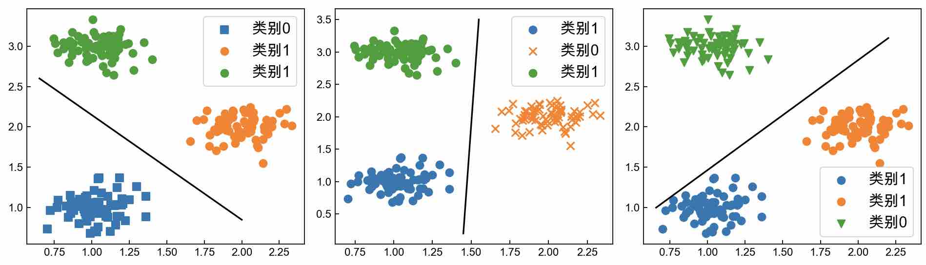
用逻辑回归处理多分类任务时,都会采用一种称为One-vs-all(也叫作 One-vs-rest)的方法,两者的缩写分别为ova与ovr。这种策略的核心思想就是每次将其中一个类和剩余的其他类看作一个二分类任务进行训练,最后在预测过程中选择输出概率值最大那个类作为该样本点所属的类别。
代码实现#
import matplotlib.pyplot as plt
import numpy as np
from sklearn.datasets import make_blobs

def visualization():
    num_points = 200
    centers = [[1, 1], [2, 2], [1, 3]]  # 指定中心
    x, y = make_blobs(n_samples=num_points, centers=centers,
                      cluster_std=0.15, random_state=np.random.seed(10))
    index_c0, index_c1, index_c2 = (y == 0), (y == 1), (y == 2)
    c0, c1, c2 = x[index_c0], x[index_c1], x[index_c2]
    plt.rcParams['ytick.direction'] = 'in'  # 刻度向内
    plt.rcParams['xtick.direction'] = 'in'  # 刻度向内
    plt.rcParams['font.sans-serif'] = ['SimHei']  # 指定默认字体
    plt.tick_params(axis='x', labelsize=15)  # x轴刻度数字大小
    plt.tick_params(axis='y', labelsize=15)  # y轴刻度数字大小
    plt.scatter(c0[:, 0], c0[:, 1], marker='s', label='类别0', s=50)
    plt.scatter(c1[:, 0], c1[:, 1], marker='x', label='类别1', s=50)
    plt.scatter(c2[:, 0], c2[:, 1], marker='v', label='类别2', s=50)
    plt.legend(fontsize=15)
    plt.tight_layout()
    plt.show()

def visualization_ova():
    plt.figure(figsize=(12, 3.5), dpi=80)
    plt.subplot(1, 3, 1)
    num_points = 200
    centers = [[1, 1], [2, 2], [1, 3]]  # 指定中心
    x, y = make_blobs(n_samples=num_points, centers=centers,
                      cluster_std=0.15, random_state=np.random.seed(10))
    index_c0, index_c1, index_c2 = (y == 0), (y == 1), (y == 2)
    c0, c1, c2 = x[index_c0], x[index_c1], x[index_c2]
    plt.rcParams['ytick.direction'] = 'in'  # 刻度向内
    plt.rcParams['xtick.direction'] = 'in'  # 刻度向内
    # plt.rcParams['font.sans-serif'] = ['Arial Unicode MS']
    plt.rcParams['font.sans-serif'] = ['SimHei']  # 指定默认字体
    plt.tick_params(axis='x', labelsize=15)  # x轴刻度数字大小
    plt.tick_params(axis='y', labelsize=15)  # y轴刻度数字大小
    plt.scatter(c0[:, 0], c0[:, 1], marker='s',  label='类别0', s=50)
    plt.scatter(c1[:, 0], c1[:, 1], marker='o',  label='类别1', s=50)
    plt.scatter(c2[:, 0], c2[:, 1], marker='o',  label='类别1', s=50)
    plt.plot([0.65, 2.0], [2.6, 0.85], c='black')
    plt.legend(fontsize=15)

    plt.subplot(1, 3, 2)
    num_points = 200
    centers = [[1, 1], [2, 2], [1, 3]]  # 指定中心
    x, y = make_blobs(n_samples=num_points, centers=centers,
                      cluster_std=0.15, random_state=np.random.seed(10))
    index_c0, index_c1, index_c2 = (y == 0), (y == 1), (y == 2)
    c0, c1, c2 = x[index_c0], x[index_c1], x[index_c2]
    plt.rcParams['ytick.direction'] = 'in'  # 刻度向内
    plt.rcParams['xtick.direction'] = 'in'  # 刻度向内
    # plt.rcParams['font.sans-serif'] = ['Arial Unicode MS']
    plt.rcParams['font.sans-serif'] = ['SimHei']  # 指定默认字体
    plt.tick_params(axis='x', labelsize=15)  # x轴刻度数字大小
    plt.tick_params(axis='y', labelsize=15)  # y轴刻度数字大小
    plt.scatter(c0[:, 0], c0[:, 1], marker='o',  label='类别1', s=50)
    plt.scatter(c1[:, 0], c1[:, 1], marker='x',  label='类别0', s=50)
    plt.scatter(c2[:, 0], c2[:, 1], marker='o',  label='类别1', s=50)
    plt.plot([1.45, 1.55], [0.2, 3.5], c='black')
    plt.legend(fontsize=15)

    plt.subplot(1, 3, 3)
    num_points = 200
    centers = [[1, 1], [2, 2], [1, 3]]  # 指定中心
    x, y = make_blobs(n_samples=num_points, centers=centers,
                      cluster_std=0.15, random_state=np.random.seed(10))
    index_c0, index_c1, index_c2 = (y == 0), (y == 1), (y == 2)
    c0, c1, c2 = x[index_c0], x[index_c1], x[index_c2]
    plt.rcParams['ytick.direction'] = 'in'  # 刻度向内
    plt.rcParams['xtick.direction'] = 'in'  # 刻度向内
    # plt.rcParams['font.sans-serif'] = ['Arial Unicode MS']
    plt.rcParams['font.sans-serif'] = ['SimHei']  # 指定默认字体
    plt.tick_params(axis='x', labelsize=15)  # x轴刻度数字大小
    plt.tick_params(axis='y', labelsize=15)  # y轴刻度数字大小
    plt.scatter(c0[:, 0], c0[:, 1], marker='o',  label='类别1', s=50)
    plt.scatter(c1[:, 0], c1[:, 1], marker='o',  label='类别1', s=50)
    plt.scatter(c2[:, 0], c2[:, 1], marker='v',  label='类别0', s=50)
    plt.plot([0.66, 2.2], [1, 3.1], c='black')
    plt.legend(fontsize=15)
    plt.tight_layout()  # 调整子图间距
    plt.show()

if __name__ == '__main__':
    visualization()
visualization_ova()运行结果#
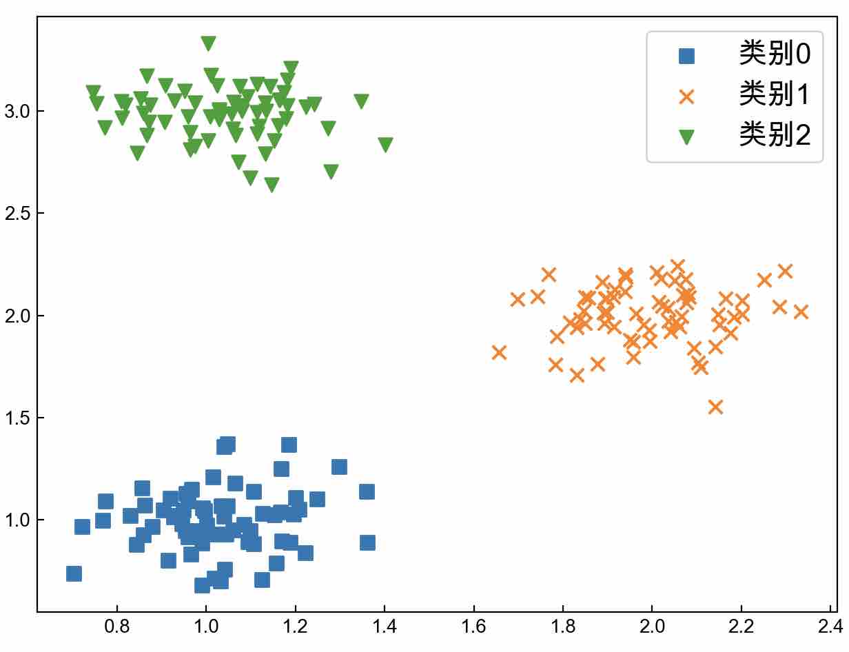
当利用One-vs-all的分类思想来解决图1中的多分类问题时,可以可视化成如图2所示的情况。
阅读
--