更新于
2026年7月26日
过拟合#
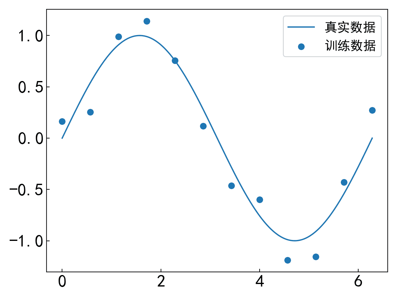
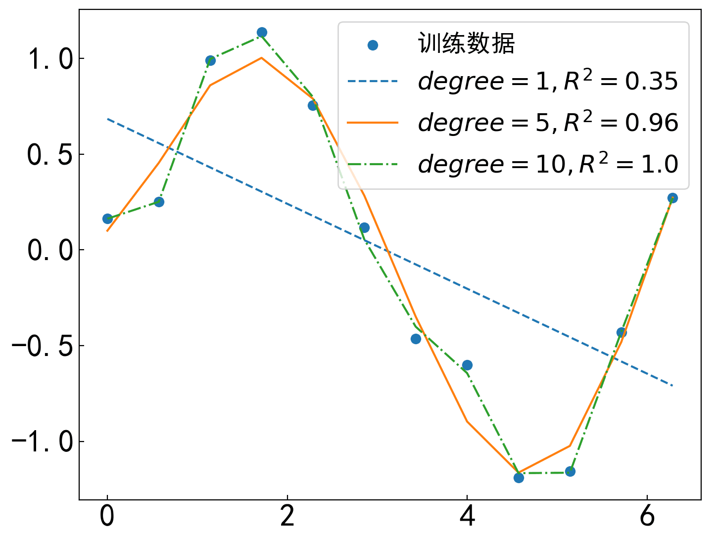
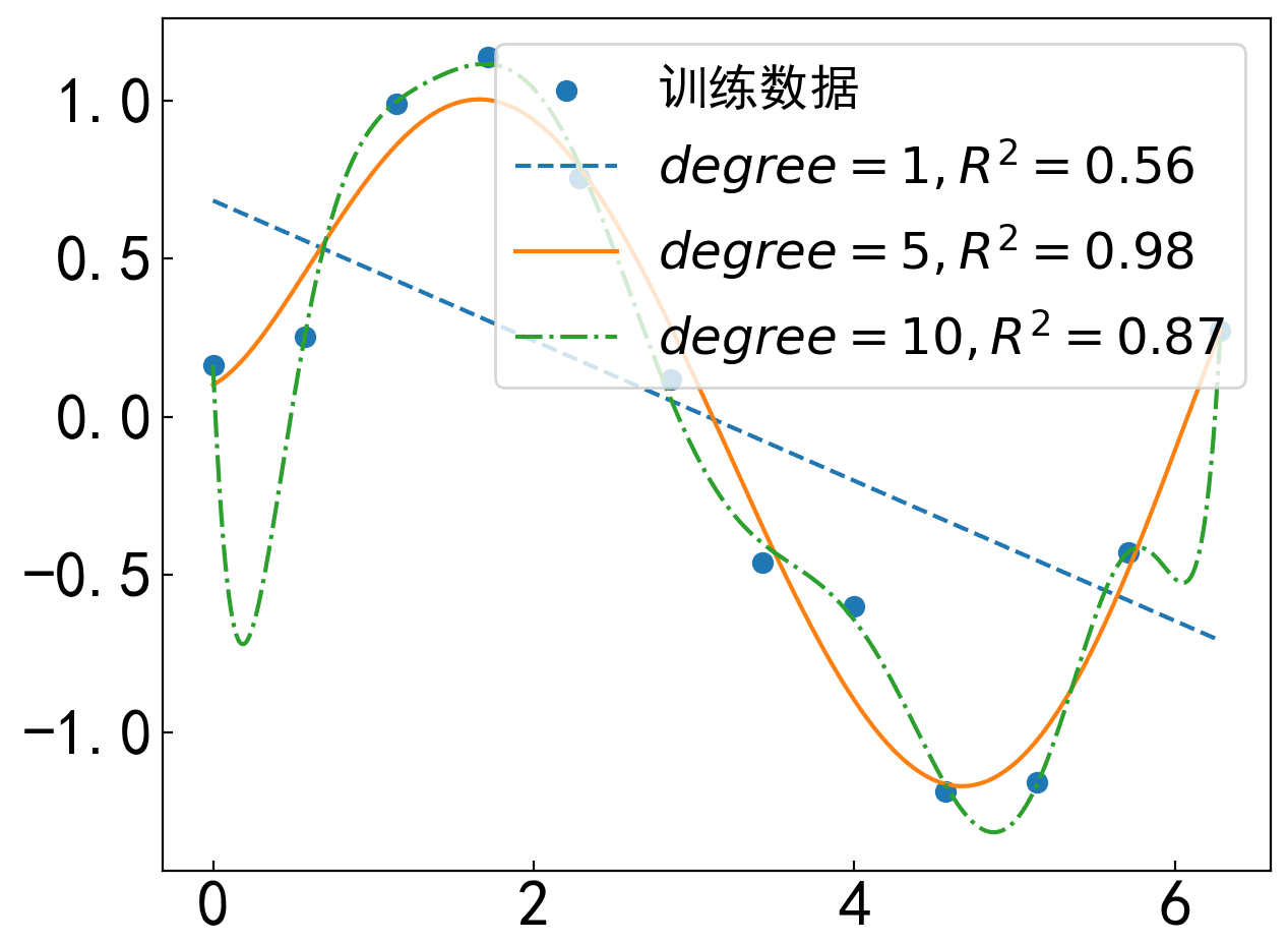
模型的参数是一步一步根据梯度下降算法更新而来,直至目标函数收敛,也就是说这是一个循序渐进的过程,因此,这一过程也被称作是拟合(Fitting)模型参数的过程,当这个过程执行结束后就会产生3种状态,即过拟合(Overfitting)、恰拟合(Goodfitting)和欠拟合(Underfitting)。
代码实现#
import matplotlib.pyplot as plt
import numpy as np
from sklearn.preprocessing import PolynomialFeatures
from sklearn.linear_model import LinearRegression

def make_data():
    np.random.seed(10)
    x_train = np.linspace(0, 2 * np.pi, 12)  # 训练样本
    x_test = np.linspace(0, 2 * np.pi, 1000)
    y_test = np.sin(x_test)
    y_train = np.random.uniform(-0.3, 0.3, 12) + np.sin(x_train)
    return x_test.reshape(-1, 1), y_test, x_train.reshape(-1, 1), y_train

def visualization(x_test, y_test, x_train, y_train):
    plt.rcParams['ytick.direction'] = 'in'  # 刻度向内
    plt.rcParams['xtick.direction'] = 'in'  # 刻度向内
    plt.rcParams['font.sans-serif'] = ['SimHei']  # 指定默认字体
    plt.rcParams['axes.unicode_minus'] = False
    plt.tick_params(axis='x', labelsize=20)  # x轴刻度数字大小
    plt.tick_params(axis='y', labelsize=20)  # y轴刻度数字大小
    plt.plot(x_test, y_test, label='真实数据', )
    plt.scatter(x_train, y_train, label='训练数据', s=45)
    plt.tight_layout()  # 调整子图间距
    plt.legend(fontsize=15)
    plt.show()

def polynomial_regression(x_train, y_train, x_test, y_test, degree=2):
    poly = PolynomialFeatures(include_bias=False, degree=degree)
    x_mul = poly.fit_transform(x_train)
    model = LinearRegression()

    model.fit(x_mul, y_train)

    x_mul = poly.transform(x_test)
    y_pre = model.predict(x_mul)
    r2 = model.score(x_mul, y_test)
    return y_pre, r2

def prediction(x_test, y_test, x_train, y_train):
    y_pre_1, r2_1 = polynomial_regression(x_train, y_train, x_test, y_test, degree=1)
    y_pre_5, r2_5 = polynomial_regression(x_train, y_train, x_test, y_test, degree=5)
    y_pre_10, r2_10 = polynomial_regression(x_train, y_train, x_test, y_test, degree=10)
    plt.rcParams['ytick.direction'] = 'in'  # 刻度向内
    plt.rcParams['xtick.direction'] = 'in'  # 刻度向内
    plt.rcParams['font.sans-serif'] = ['SimHei']  # 指定默认字体
    plt.rcParams['axes.unicode_minus'] = False
    plt.tick_params(axis='x', labelsize=23)  # x轴刻度数字大小
    plt.tick_params(axis='y', labelsize=23)  # y轴刻度数字大小
    plt.scatter(x_train, y_train, label='训练数据', s=45)
    plt.plot(x_test, y_pre_1, linestyle='--', label=r'$degree = 1, R^2 = {}$'.format(round(r2_1, 2)), )
    plt.plot(x_test, y_pre_5, label=r'$degree = 5, R^2 = {}$'.format(round(r2_5, 2)), )
    plt.plot(x_test, y_pre_10, linestyle='dashdot', label=r'$degree = 10, R^2 = {}$'.format(round(r2_10, 2)), )
    plt.tight_layout()  # 调整子图间距
    plt.legend(fontsize=18, loc='upper right')
    plt.show()


def train(x_train, y_train):
    y_pre_1, score_1 = polynomial_regression(x_train, y_train, x_train, y_train, degree=1)
    y_pre_5, score_5 = polynomial_regression(x_train, y_train, x_train, y_train, degree=5)
    y_pre_10, score_10 = polynomial_regression(x_train, y_train, x_train, y_train, degree=10)

    plt.scatter(x_train, y_train, label='训练数据', s=45)
    plt.plot(x_train, y_pre_1, linestyle='--', label=r'$degree = 1, R^2 = {}$'.format(round(score_1, 2)), )
    plt.plot(x_train, y_pre_5, label=r'$degree = 5, R^2 = {}$'.format(round(score_5, 2)), )
    plt.plot(x_train, y_pre_10, linestyle='dashdot',
             label=r'$degree = 10, R^2 = {}$'.format(round(score_10, 2)), )
    plt.rcParams['font.sans-serif'] = ['SimHei']  # 指定默认字体
    plt.tick_params(axis='x', labelsize=23)  # x轴刻度数字大小
    plt.tick_params(axis='y', labelsize=23)  # y轴刻度数字大小
    plt.rcParams['axes.unicode_minus'] = False
    plt.legend(fontsize=18, loc='upper right')
    plt.tight_layout()  # 调整子图间距
    plt.show()


if __name__ == '__main__':
    x_test, y_test, x_train, y_train = make_data()
    visualization(x_test, y_test, x_train, y_train)  # 可视化训练样本
    train(x_train, y_train)  # 可视化拟合后的曲线
prediction(x_test, y_test, x_train, y_train) # 预测新样本的输出运行结果#
阅读
--