模型蒸馏在 BERT 上的应用，DistilBERT 原理与实现过程！ • 《从零学AI指南手册》

更新于 2026年7月7日

在上一篇文章「模型蒸馏的原理是什么？温度有什么用？起底LLM中的蒸馏技术！」中，我们详细介绍了模型蒸馏（Distillation）的原理，并且还通过下面这张图来辨析了模型迁移和模型蒸馏的区别之处。

图 1. 模型迁移与模型蒸馏

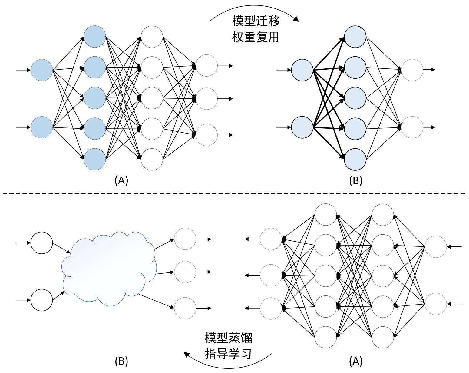
简单来讲，模型迁移是将模型的 A 的部分或全部能力迁移到模型 B 中，而迁移的过程本质上就是将用 A 中的权重参数来重新初始化 B 中对应的权重参数，这也就暗含着迁移部分的网络结构是一样；而模型蒸馏则更像是拿复杂模型 A 来作为一个超牛逼的老师，然后来指导学生模型 B 的训练使得它能够模仿输出和复杂模型类似的结果，两者的网络结构可以是截然不同的。

掌柜刚说完在模型蒸馏中教师模型和学生模型的网络结构可以是截然不同的，这里立马就来了个抄作业的家伙，基于 BERT 蒸馏而来的 DistilBERT。当然，理解本文的前提是需要先了解 BERT 的基本原理，具体可以参见本专栏中的相关文章。

在 DistilBERT 中，为了让学生模型学得更快一点，它干脆直接抄起了老师模型的作业，通过直接使用教师模型中的部分权重参数来初始化学生模型中的权重参数，这也就意味着学生模型抄作业部分的网络结构和教师模型是一致的。

当然，人家 DistilBERT 也没有直接原封不动地抄，还是用了一定的策略，不然作业交上去铁定被发现。

关键词：模型迁移、模型蒸馏、DeepSeek、DistilBERT、BERT

1. DistilBERT 提出动机#

经过上一篇文章的介绍，相信大家对于模型蒸馏的思想及原理已经有了比较清晰的认识。接下来掌柜就来带着大家看看 DistilBERT[1] 提出的动机以及它具体的技术原理。

随着自然语言技术的快速发展，尤其是预训练范式的出现，使得将相关模型部署到边缘计算设备上的成本急剧增加。在这样的背景下，Hugging Face 提出了基于 BERT 模型蒸馏而来的 DistilBERT 模型。

these large models in on-the- edge and/or under constrained computational training or inference budgets remains challenging.

图 2. 模型发展带来的参数量变化情况

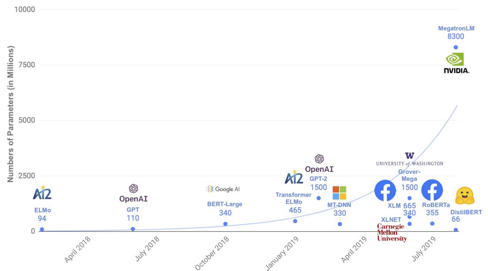
从图1中可以看出，尽管后来的模型效果上取得了显著的提升，但是参数量却迎来了剧烈的激增，并且研究显示随着参数量的增加模型的效果还能更好（当时作者这样的预言随着后来GPT-3和ChatGPT等的出现也得到了完美的验证）。这也就暗示着必须要通过某种办法来控制模型参数的大规模增长。

While these models lead to significant improvement, they often have several hundred million parameters and current research on pre-trained models indicates that training even larger models still leads to better performances on downstream tasks.

尽管在此之前已经有研究者在特定场景任务下来对模型进行蒸馏，即随机初始化权重通过学生模型学习教师模型的输出分布来训练模型，这也是模型蒸馏的标准做法。但是 Hugging Face 则采取了另外一种方式，即在预训练阶段开始便对 BERT 模型进行蒸馏，同时还将教师模型（原始 BERT）中的部分权重参数迁移到了学生模型（DistilBERT模型）中。最后，相比较于原始的 BERT 模型，DistilBERT 在参数量上减少了 40% 但是保留了 97% 的语言理解能力，且提高了 60% 的运行速度。

While most prior work investigated the use of distillation for building task-specific models, we leverage knowledge distillation during the pre-training phase and show that it is possible to reduce the size of a BERT model by 40%, while retaining 97% of its language understanding capabilities and being 60% faster.

图 3. DistilBERT 实验结果

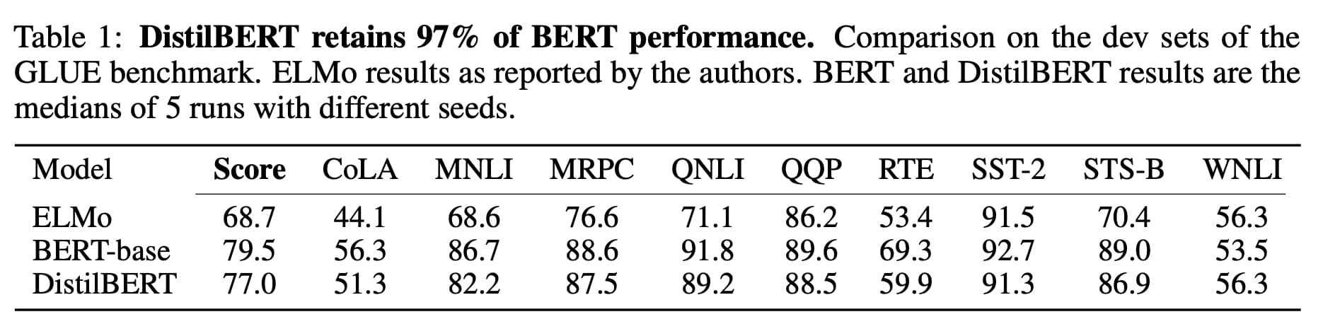
这里细想一想，其实 DistilBERT 更像是模型迁移与模型蒸馏这两项技术结合一个产物。

2. DistilBERT 原理#

在清楚 DistilBERT 的提出动机后我们再来看一下它的具体构建原理。从整体来看，DistilBERT 的蒸馏过程涉及两个方面：①损失函数由三部分构成

② 学生模型的初始化权重来源于教师模型中的网络权重。

2.1 DistilBERT 中的损失函数#

我们知道，当一个模型在训练集上表现良好时，也就意味着它的输出分布通常会在正确类别上给出很高的概率，而对于其他类别则会给出接近于零的概率。然而，尽管这些 “接近零” 的概率很小，但是它们之间仍有差异，而这对于模型蒸馏来说却是非常重要的。因为这些差异部分便反映了模型在未知样本上的泛化能力，以及它在测试集上的表现。如果模型能够给出较小概率的类别之间有区分度，这可能意味着它能够更好地识别数据中的细微差异，而不仅仅是对训练集所出现情况的简单记忆。

A model performing well on the training set will predict an output distribution with high probability on the correct class and with near-zero probabilities on other classes. But some of these “near-zero” probabilities are larger than others and reflect, in part, the generalization capabilities of the model and how well it will perform on the test set.

例如对于如下示例来说可以利用 BERT 来完成对其中 [MASK] 不分的预测。

I think this is the beginning of a beautiful [MASK].

根据对这句话上下文语境的理解，模型可能会对 “day” and “life” 这个两个词给出很高的概率，但同时也会给 “future”, “story”, “world”… 这样的词（称为长尾词）给出较小的概率。前者表示这两个词在该上下文中非常合适，并且模型对这两个词的信心很高；后者表示虽然这些词的概率较低，但它们依然是合适的候选词，并且在某些上下文中也能使句子变得合理。

简单来讲，如果模型给 “day” and “life” 这两个词的概率加起来为1，其它所有词的概率为0，那么我们可以合理的怀疑模型仅仅只是记住了训练集中所出现的情境，而毫无泛化能力。所以，这种高概率和低概率的词汇差异意味着 BERT 不仅仅是“记住”训练数据中的固定模式，而是能够理解语言的丰富性和多样性，这种能力使得它在面对未见过的文本时，能够灵活地做出预测，而不仅仅是过度依赖某些显而易见的答案。

因此，在很多自然语言处理任务中，尤其是生成任务中，长尾词的有效预测是非常重要的。它展示了模型对于不同但合理的答案的潜在理解和预测能力，即使对于某些词，模型的信心较低（概率较小），它依然能够提出多个合理的答案，这正是模型的多样性和泛化能力的体现。

因此，可以再次看出在模型蒸馏中，教师模型的输出概率分布相较于单一的独热编码标签，能够提供更多丰富的信息。

2.1.1 硬交叉熵损失原理#

在模型蒸馏中，除了教师模型和学生模型之间的软交叉熵以外，还有一部分就是学生模型与真实标签之间的硬交叉熵，即 $L_{mlm}$ 。在原始的 BERT 模型中这部分由两块构成，一个是 NSP 任务，一个是 MLM 任务。但是在 DistilBERT 中，作者仅保留了最重要的 MLM 来对模型进行蒸馏。原理这里就不再赘述，大家可以参见专栏第10.6节内容。

2.1.2 软交叉熵损失原理#

在 DistilBERT 中，损失函数中的第二部分依旧是教师模型的输出概率分布 $t_i$ 与学生模型输出概率分布 $s_i$ 之间的交叉熵，即

$$ L_{ce}=\sum_{i}t_i\log(s_i)\tag{1} $$

当然，同「上一篇」文章中我们介绍的计算过程一样，$t_i$ 和 $s_i$ 也是经过式(2)计算后的结果。

$$ p_i=\frac{\exp(z_i/T)}{\sum_j\exp(z_j/T)}\tag{2} $$

更多细节可以参见上一篇文章。

2.1.3 余弦距离损失原理#

除了模型整理中比较常见的软交叉熵和硬交叉熵损失以外，DistilBERT 中还加入了一种新的余弦嵌入损失（Cosine Embedding Loss），即 $L_{cos}$ 。余弦嵌入损失的目标是最小化这种损失，促使学生模型的隐藏状态向量与教师模型的向量在方向上尽可能相似或对齐，这有助于学生模型更好地模仿教师模型的表示能力，而不仅仅是输出结果。

具体来说，余弦相似度计算的是两个向量夹角的余弦值，值范围在 -1 到 1 之间。1 表示两个向量的方向完全一致夹角为0度；-1 表示两个向量方向完全相反夹角为180度；0 表示两者正交没有方向上的相似性夹角为90度。余弦距离则是根据余弦相似度人为构建出来的一种距离。从直观上看，越相似的两个向量距离应该越近，反之越远，因此余弦距离可以表示为1减去余弦相似度。计算公式如下所示：

$$ \text{loss}(x_1,x_2) =1 - \cos(x_1, x_2) \tag{3} $$

The final training objective is a linear combination of the distillation loss $L_{ce}$ with the supervised training loss, in our case the masked language modeling loss $L_{mlm}$ [Devlin et al., 2018]. We found it beneficial to add a cosine embedding loss ($L_{cos}$) which will tend to align the directions of the student and teacher hidden states vectors.

最后，作者通过消融实验发现，目标函数中的每一项对于模型最后的结果都有着重要的影响。

Further ablation studies indicate that all the components of the triple loss are important for best performances.

别说，新引入的余弦损失还真是一个很新颖的视角，即使学生模型输出的向量和教师模型输出向量会在相同输入下输出的值不一样，如果我们能约束方向上的一致性，那么也能够使得学生模型的输出更加接近于教师模型。

2.2 DistilBERT 网络结构初始化#

之所以一开始掌柜就说 DistilBERT 更像是模型迁移与模型蒸馏这结合的产物，那是因为这小子它不讲武德你知道吗？不讲武德。

明明说好了靠蒸馏来训练模型，结果它还直接抄了部分作业，把人家 BERT 中一半的权重参数直接抄过来了。

2.2.1 网络结构#

从名字也可以看出， DistilBERT 的网络整体结构同 BERT 类似，唯一的两点区别在于：① DistilBERT 中去掉了 token-type embeddings （即用于区分两个句子的句子编码）和最后一个 bert pooler 层。② DistilBERT 整体的网络层数相较于 BERT 减半，这是因为作者研究发现，在同样参数量的情况下，层数减半的效果更好。

The token-type embeddings and the pooler are removed while the number of layers is reduced by a factor of 2. Most of the operations used in the Transformer architecture (linear layer and layer normalisation) are highly optimized in modern linear algebra frameworks and our investigations showed that variations on the last dimension of the tensor (hidden size dimension) have a smaller impact on computation efficiency (for a fixed parameters budget) than variations on other factors like the number of layers. Thus we focus on reducing the number of layers.

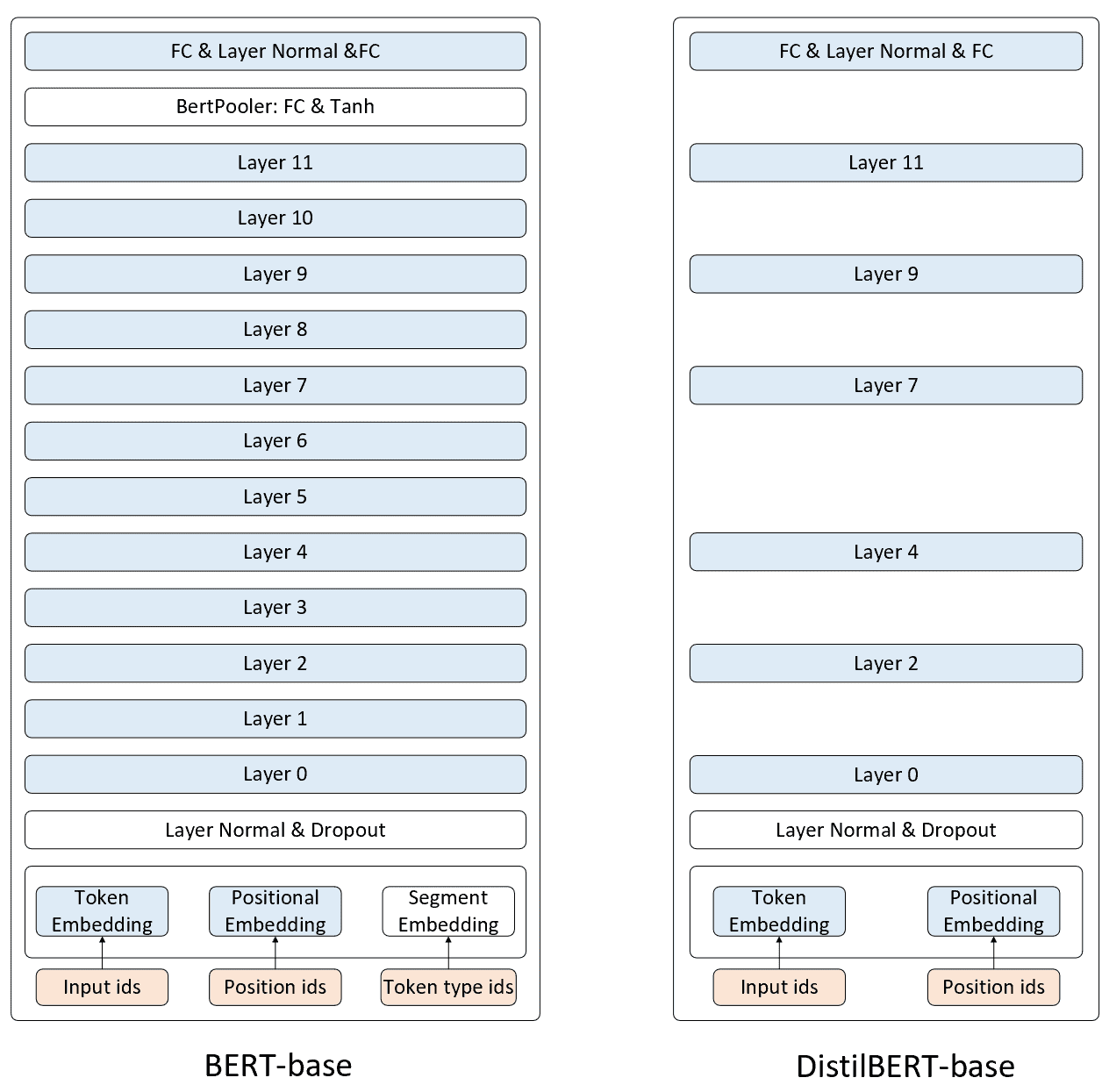
图 4. BERT-base 与 DistilBERT-base 网络结构对比图

如图3所示便是BERT-base 与 DistilBERT-base 网络结构对比图，其中蓝色部分表示被迁移的权重参数，不过最上面一层 LN 中的权重参数为迁移，此处只是为了画图方面。

可以看出，DistilBERT-base 并不是直接取 BERT-base 中的前6层或者后6层，而是整体上以2为倍数进行抽取作为初始化 DistilBERT-base 的参数。

下表所示便是以 BERT-base 为例进行蒸馏时 DistilBERT-base 的网络结构参数对比情况。可以发现，整体网络结构类似，仅仅是层数进行了减半处理。

BERT-base	DistilBERT-base
hidden_size = 768	dim = 768
intermediate_size = 3072	hidden_dim = 3072
max_position_embeddings = 512	max_position_embeddings = 512
num_attention_heads = 12	n_heads = 12
num_hidden_layers = 12	n_layers = 6
vocab_size = 30522	vocab_size = 30522

2.2.2 权重初始化#

具体来说，DistilBERT-base 是以 BERT-base 的预训练模型为基础，然后将 BERT-base 中word_embedding、position_embeddings以及第 [0, 2, 4, 7, 9, 11] 层的代码迁移到了 DistilBERT-base 中。

3. DistilBERT 使用与实现#

DistilBERT 是由 Hugging Face 所提出，因此我们可以直接通过 Transformers 库中的对应模块来进行使用。接下来掌柜将分别介绍如何使用 Transformers 库中 DistilBERT 来完成诸如文本分类这样简单的下游任务，以及蒸馏过程的实现。

3.1 基于 DistilBERT 的下游任务#

基于 DistilBERT 的的下游任务和 BERT 模型一样，只需要拿到前向传播结束后的输出向量进行损失计算训练或者推理即可，示例代码如下：

 1 from transformers import DistilBertTokenizer, DistilBertModel, DistilBertConfig
 2 import torch.nn as nn
 3 import torch
 4 
 5 class DistilBertSentenceClassification(nn.Module):
 6     def __init__(self, config: DistilBertConfig):
 7        1 super(DistilBertSentenceClassification, self).__init__()
 8         self.distilbert = DistilBertModel.from_pretrained("./distilbert_base_uncased")
 9         self.pre_classifier = nn.Linear(config.dim, config.dim)
10         self.classifier = nn.Linear(config.dim, config.num_labels)
11         self.dropout = nn.Dropout(config.seq_classif_dropout)
12         self.num_labels = config.num_labels
13 
14     def forward(self, input_ids=None, attention_mask=None, labels=None):
15         distilbert_output = self.distilbert(input_ids=input_ids, attention_mask=attention_mask)
16         hidden_state = distilbert_output[0]  # [batch_size, seq_len, dim]
17         pooled_output = hidden_state[:, 0]  # [batch_size, dim]
18         pooled_output = self.pre_classifier(pooled_output)  # [batch_size, dim]
19         pooled_output = nn.ReLU()(pooled_output)  # [batch_size, dim]
20         pooled_output = self.dropout(pooled_output)  # [batch_size, dim]
21         logits = self.classifier(pooled_output)  # [batch_size, num_labels]
22         if labels is not None:
23             loss_fct = nn.CrossEntropyLoss()
24             loss = loss_fct(logits.view(-1, self.num_labels), labels.view(-1))
25             return loss, logits
26         else:
27             return logits

在上述代码中，第8行便是通过本地的权重参数实例化一个 DistilBertModel 模型。第15~16行是取 DistilBertModel 前向传播后的结果，后续则是相应的分类或损失计算流程不再赘述。上述完整示例代码可参见 Code/C01_Distillation/C03_DistilBert/distilbert_tasks.py 文件。

3.2 DistilBERT 模型蒸馏#

在介绍完如何利用 Transformers 框架以后，我们再来看如何动手实现 DistilBERT 训练部分的代码。由于整个数据集的构建过程同 BERT 预训练中的一致，所以这里就不再赘述大家直接参考本专栏第10.12节中的实现使用即可。下面掌柜着重来介绍一下如何构建 DistilBERT 中三个部分的损失。

3.2.1 硬交叉熵损失实现#

这部分损失是最简单的，直接使用 DistilBERT 最后一层的输出，同正确标签计算损失值即可。在实现这部分代码以前，我们先来构建一个辅助函数帮助我们得到教师模型和学生模型，示例代码如下：

1 def get_teacher_student_models():
2     teacher_model = BertForMaskedLM.from_pretrained('./bert_base_uncased')
3     teacher_model.eval()
4     student_model = DistilBertForMaskedLM.from_pretrained(
5                                     './distilbert_from_bert_base_uncased')
6     return teacher_model, student_model

在上述代码中，第2行是得到一个根据本地权重参数实例化后的 BertForMaskedLM 模型。第4~5行则是读取从 bert_base_uncased 这个模型中筛选出来的权重参数实例化到本地后，在将其用来初始化 DistilBertForMaskedLM 中的权重参数。因此，我们需要先运行工程中的 extract_distilbert.py 函数，来将 bert_base_uncased 中的参数按照上面第2.2节介绍的策略进行抽取，并保存到当前目录的 distilbert_from_bert_base_uncased文件夹下。第6行则是返回两个实例化后的教师模型和学生模型。

进一步，我们来构建几个模拟的样本，以用于测试后续代码。

1 if __name__ == '__main__':
2     teacher_model, student_model = get_teacher_student_models()
3     input_ids = torch.tensor([[5, 1414, 232, 328, 0],
4                     [1, 56, 34, 0, 0]], dtype=torch.int32)
5     hard_label = torch.tensor([[-100, 1414, -100, 328, -100],  # -100 表示不参与损失计算
6                     [1, -100, 34, -100, -100]], dtype=torch.long)
7     attention_mask = torch.tensor([[1, 1, 1, 1, 0],
8                     [1, 1, 1, 0, 0]], dtype=torch.long)  # [batch_size, seq_len]
9     temperature = 2.

在上述代码中，第3~4行是构建两个样本，其中 0 表示该位置为填充值（默认情况下现在开源的模型 pad_idx 都是 0 ）。第5~6行则是构建两个样本在 MLM 任务重对应的标签值，这里尤其需要注意的一点是，由于我们这里使用的是 DistilBertForMaskedLM 模块来完成损失的计算，而它并不支持手动指定 nn.CrossEntropyLoss() 中的 ignore_index，因此我们在构建数据集的时候，要将需要忽略计算损失部分的 token id 设置为 -100，因为 -100 是 nn.CrossEntropyLoss() 中 ignore_index 的默认值。第7~8行则是构造掩码向量，本质上是 key_padding_mask ，形状为 [batch_size, seq_len]，其中为 0 的位置后续计算注意力的时候会被忽略。

1     s_results = student_model(input_ids, attention_mask=attention_mask, 
2                               labels=hard_label, output_hidden_states=True, )
3     s_mlm_loss, s_logits  = s_results.loss, s_results.logits
4     s_hidden_states = s_results.hidden_states[-1]

在上述代码中，第1~2行是使用学生模型来计算得到前向传播的输出结果。第3行便是取学生模型 MLM 任务的损失以及对应的 logits 值，后者形状是 [batch_size, seq_len, vocab_size]，因为后续要同教师模型的 logits 进行损失计算。第4行是注意力层最后一层的输出，形状是 [batch_size, seq_len, dim]。

3.2.2 软交叉熵损失实现#

紧接着我们开始计算软交叉熵损失。由于在序列任务预测中我们需要考虑padding填充的情况，即填充部分的损失我们忽略掉，因此在根据式(1)计算软交叉熵之前我们需要对学生模型和教师模型输出的 logits 分别进行过滤，即只保留那些非填充位置上的 logits 值。这里我们会用到 torch.masked_select() 方法来进行筛序。

不过有朋友可能会问，为啥不使用指定 ignore_idx 的方式来忽略这部分损失？

那是因为在计算 soft loss 的时候，没有硬标签，不能明确知道那个位置上的损失是可以被忽略的，所以不能通过指定 ignore_idx 的方式来进行忽略，必须通过手动根据 attention_mask 进行筛选。示例代码如下所示：

 1     with torch.no_grad():
 2         t_result = teacher_model(input_ids, attention_mask=attention_mask,
 3                                  output_hidden_states=True, output_attentions=True)
 4         t_logits, t_hidden_states = t_result.logits, t_result.hidden_states[-1]
 5 
 6     mask = attention_mask.unsqueeze(-1).expand_as(s_logits) == 1 
 7     s_logits_slc = torch.masked_select(s_logits, mask)
 8     s_logits_slc = s_logits_slc.view(-1, s_logits.size(-1)) 
 9     t_logits_slc = torch.masked_select(t_logits, mask)  
10     t_logits_slc = t_logits_slc.view(-1, s_logits.size(-1))
11     loss_soft = nn.functional.kl_div(F.softmax(s_logits_slc / temperature, dim=-1),
12               F.softmax(t_logits_slc / temperature, dim=-1), reduction='batchmean')
13     loss_soft = loss_soft * temperature ** 2

在上述代码中，第1~4行是根据输入获取得到教师模型的 logits 和多层多头注意力最后一层的输出 t_hidden_states，其形状分别为 [batch_size, seq_len, vocab_size] 和 [batch_size, seq_len, dim]，根据上面给出的示例输出结果则为 [2, 5, 30522] 和 [2, 5, 768]。

第6行则是根据 attention_mask 得到一个用于下面筛选 s_logits 中不是填充部分的值。这里需要注意的一点是，masked_select 函数只接受布尔值，所以这里通过 ==1 来判断得到 attention_mask 的结果。

下面看一个简单的示例。

1     s_hidden_states = torch.randn([2, 5, 4])
2     t_hidden_states = torch.randn([2, 5, 4]) 
3     attention_mask = torch.tensor([[True, True, True, True, False], 
4                                [True, True, False, False, False]])
5     mask = attention_mask.unsqueeze(-1).expand_as(s_hidden_states)

对于上述代码来说，attention_mask 的形状为 [2, 5]，最后 mask 的输出结果为

 1 tensor([[[ True,  True,  True,  True],
 2          [ True,  True,  True,  True],
 3          [ True,  True,  True,  True],
 4          [ True,  True,  True,  True],
 5          [False, False, False, False]],
 6 
 7         [[ True,  True,  True,  True],
 8          [ True,  True,  True,  True],
 9          [False, False, False, False],
10          [False, False, False, False],
11          [False, False, False, False]]])

上述结果形状同 s_hidden_states 一致，为 [2, 5, 4]。通过这个 mask 向量便可以清晰地知道 s_hidden_states 和 t_hidden_states 中哪些位置上的值是不需要的。例如对于 s_hidden_states 来说，根据 attention_mask 可知其序列最后一个 token 位置上的值需要被忽略，那么对应维度上则是最后一个 token 表示的这个 4 维向量不需要，那么 mask[0][4] 这一行刚好全是 False。

进一步，继续筛选：

1     dim = s_hidden_states.size(-1)
2     s_hidden_states_slct = torch.masked_select(s_hidden_states, mask)
3     s_hidden_states_slct = s_hidden_states_slct.view(-1, dim)

上述代码中，s_hidden_states_slct 是根据 mask 向量筛选 s_hidden_states 而来。此时，s_hidden_states 的结果为：

 1 tensor([[[ 0.2609, -0.3028, -0.7821,  1.0134],
 2          [ 1.0945, -0.5793, -1.0508, -0.3901],
 3          [ 0.0562, -0.9556, -0.3812, -0.7870],
 4          [ 0.4945, -0.3497,  0.4294,  0.5628],
 5          [-1.3939, -0.6685, -0.4936,  0.8770]],
 6 
 7         [[ 1.0229,  0.0375, -0.8171, -0.2017],
 8          [ 0.6605, -2.1136, -1.2689, -0.3926],
 9          [-0.4158,  0.5357, -0.7426, -0.1218],
10          [ 0.7229, -0.3661,  1.2451,  1.6738],
11          [ 0.5723, -1.4258,  0.3095,  1.3624]]])

在经过 masked_select 操作后，结果为

1 tensor([ 0.2609, -0.3028, -0.7821,  1.0134,  1.0945, -0.5793, -1.0508, -0.3901,
2          0.0562, -0.9556, -0.3812, -0.7870,  0.4945, -0.3497,  0.4294,  0.5628,
3          1.0229,  0.0375, -0.8171, -0.2017,  0.6605, -2.1136, -1.2689, -0.3926])

此时上述结构输出的是个张量列表。例如前16个元素就是第1个样本前 4 个 token 对应的 4 个向量；后 8 个元素就是第 2 个样本前 2 个 token 对应的2个向量。进一步，view 操作则是将其变形为 [6, 4]，含义则是 6 个 token 每个 token 对应一个 4 维向量。

这里把整个计算逻辑介绍清楚以后，我们再来看第3.2.2节中的第一块代码。在第11~12行计算软交叉熵时，此时 s_logits_slc 和 t_logits_slc 的形状均为 [7, 30522]，其中 7 的含义便是有 7 个有效向量。进一步，第13行便是得到最后的软交叉熵损失，原理上一篇文章中介绍过，这里就不再赘述。

3.2.3 余弦距离损失现实#

在计算余弦距离损失的时候，我们可以借助 CosineEmbeddingLoss 来实现，具体示例代码如下：

 1     cosine_loss_fct = nn.CosineEmbeddingLoss(reduction='mean')
 2     mask = attention_mask.unsqueeze(-1).expand_as(s_hidden_states) == 1
 3     dim = s_hidden_states.size(-1) 
 4     s_hidden_states_slc = torch.masked_select(s_hidden_states, mask)
 5     s_hidden_states_slc = s_hidden_states_slc.view(-1, dim)
 6     t_hidden_states_slc = torch.masked_select(t_hidden_states, mask)
 7     t_hidden_states_slc = t_hidden_states_slc.view(-1, dim)
 8     target = torch.ones(s_hidden_states_slc.size(0))
 9     loss_cos = cosine_loss_fct(s_hidden_states_slc, t_hidden_states_slc, target)
10     total_loss = 0.2 * s_mlm_loss + 0.5 * loss_soft + 0.3 * loss_cos
11     print(total_loss)

在上述代码中，第1行是实例化得到一个余弦距离计算的类实例化对象。第2~7行是先根据 attention_mask 计算得到对应的 mask 向量，然后再重新进行变形，此处 s_hidden_states_slc 和 t_hidden_states_slc 的形状均为 [7, 768]，即两个样本10个 token 中只有7个 token 是有效的。第8行是得到一个长度为7的全1向量，target: tensor([1., 1., 1., 1., 1., 1., 1.])，目的是利用 CosineEmbeddingLoss 来计算余弦距离，当 target 都为 -1 时目的是让两个向量远离。第10行则是将三部分的损失进行加权求和，其中每一项损失前的权重系数均为超参数，此处仅为示例。最后，上述代码运行结束后便可以得到损失值。

以上完整示例代码可以参见 Code/C01_Distillation/C03_DistilBert/distilbert_train.py 文件。

¡¡行文至此，对于整个 DistilBERT 的思想原理以及其初始化和训练部分的核心逻辑掌柜就介绍完了，如果大家想自己动手蒸馏得到一个 DistilBERT 模型，可以根据上述代码进行改造。

引用#

[1] Sanh V, Debut L, Chaumond J, et al. DistilBERT, a distilled version of BERT: smaller, faster, cheaper and lighter[J]. arXiv preprint arXiv:1910.01108, 2019.

[2] https://github.com/huggingface/transformers-research-projects/tree/main/distillation

[3] https://github.com/huggingface/transformers-research-projects/blob/main/distillation/scripts/extract_distilbert.py

https://github.com/huggingface/transformers-research-projects/blob/main/distillation/distiller.py

阅读 --