经过前面几节内容的介绍,我们已经清楚了BERT模型的基本原理、如何从零实现BERT模型、如何基于BERT预训练模型来完成文本分类任务、文本蕴含任务以及问答选择任务这些下游微调任务。在接下来的这节内容中,我们将会继续介绍基于BERT预训练模型的第4个下游任务微调场景,即如何完成问题回答任务。
所谓问题回答指的就是同时给模型输入一个问题和一段描述,最后需要模型从给定的描述中预测出问题答案所在的位置(text span)。
例如:
描述:苏轼是北宋著名的文学家与政治家,眉州眉山人。
问题:苏轼是哪里人?
标签:眉州眉山人
对于这样一个问题问答任务我们应该怎么来构建这个模型呢?
在做这个任务之前首先需要明白的就是:①最终问题的答案一定是在给定的描述中;②问题再描述中的答案一定是一段连续的字符,不能有间隔。例如对于上面的描述内容来说,如果给出的问题是“苏轼生活在什么年代以及他是哪里人?”,那么模型最终并不会给出类似“北宋”和“眉州眉山人”这两个分离的答案,最好的情况下便是给出“北宋著名的文学家与政治家,眉州眉山人”这一个连续的答案。
在有了这两个限制条件后,对于这类问答任务的本质也就变成了需要让模型预测得到答案在描述中的起始位置(start position)以及它的结束位置(end position)。所以,问题最终又变成了如何在BERT模型的基础上再构建一个分类器来对BERT最后一层输出的每个Token进行分类,判断它们是否属于start position或者是end position。
8.1 任务构造原理#
正如上面所说,尽管对于看似复杂的问题回答任务场景来说,其本质上依旧可以归结为一个普普通的分类任务,只是解决这个问题的关键在于如何构建这个任务以及整个数据集。
如图8-1所示,是一个基于BERT预训练模型的问题回答模型的原理图。从图中可以看出,构建模型输入的方式就是将原始问题和上下文描述拼接成一个序列中间用[SEP]符号隔开,然后再分别输入到BERT模型中进行特征提取。在BERT编码完成后,再取最后一层的输出对每个Token进行分类即可得到start position和end position的预测输出。
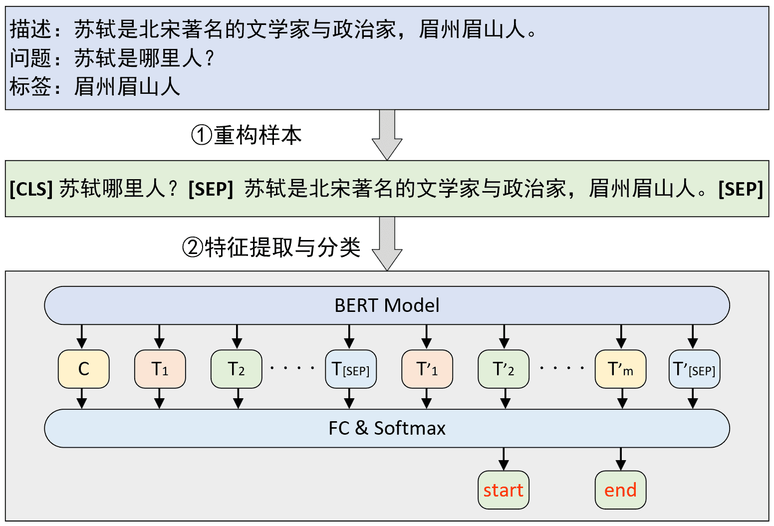
值得注意的是在问题回答场景中是将问题放在上下文描述前面的,即Sentence A为问题,Sentence B为描述[1]。而在上一个问题选择任务场景中是将答案放在描述之后。 我们猜测这是因为在SWAG这一推理数据集中,每个选项其实都可以看作是问题(描述)的下半句,两者具有强烈的先后顺序算是一种逻辑推理,因此将选项放在了描述了后面。在问题回答这一场景中,论文中将问题放在描述前面我们猜测是因为:①两者并没有强烈的先后顺序;②问题相对较短放到前面可能好处理一点。所以基于这样的考虑,在问答任务中将问题放在了描述前面。不过后续大家依旧可以尝试交换一下顺序看看效果。
到此,对于问题回答模型的原理我们算是大致清楚了,下面首先来看如何构造数据集。
8.2 数据预处理#
8.2.1 输入介绍#
在正式介绍如何构建数据集之前我们先来看这么一个问题以及其对应的常见解决方案。如果在建模时碰到上下文过长时的情况该怎么办?是直接采取截断处理吗?如果问题答案恰巧是在被截断的那部分里面呢,还能直接截断吗?显然,认真想一想截断这种做法在这里肯定是不行的,因此在论文中作者也采用了另外一种方法来解决这一问题,那就是滑动窗口。
在问题回答这个任务场景中(其它场景也可以参考借鉴),当原始的上下文过长超过给定长度或者是512个字符时,可以采取滑动窗口的方法来构造整个模型的输入序列,如图8-2所示。
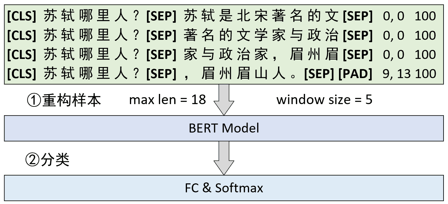
在图8-2所示的这一场景中,第①步需要做的是根据指定最大长度和滑动窗口大小将原始样本进行滑动窗口处理并得到多个子样本。不过这里需要注意的是,sentence A,也就是问题部分不参与滑动处理。同时,图8-2中样本右边的3列数字分别表示每个子样本的起始结束索引和原始样本对应的ID。紧接着第②步便是将所有原始样本滑动处理后的结果作为训练集来训练模型。
总的来说,在这一场景中训练程并没有太大的问题,因为每个子样本也都有其对应的标签值,因此和普通的训练过程并没有什么本质上的差异。因此,最关键的地方在于如何在推理过程中也使用滑动窗口。
8.2.2 结果筛选#
一种最直观的做法就是直接取起始位置预测概率值加结束位置预测概率值最大的子样本对应的结果,作为整个原始样本对应的预测结果。不过下面我们将来介绍另外一种效果更好的处理方式(这也是论文中所采取的方式),其整个处理流程如图8-3所示。
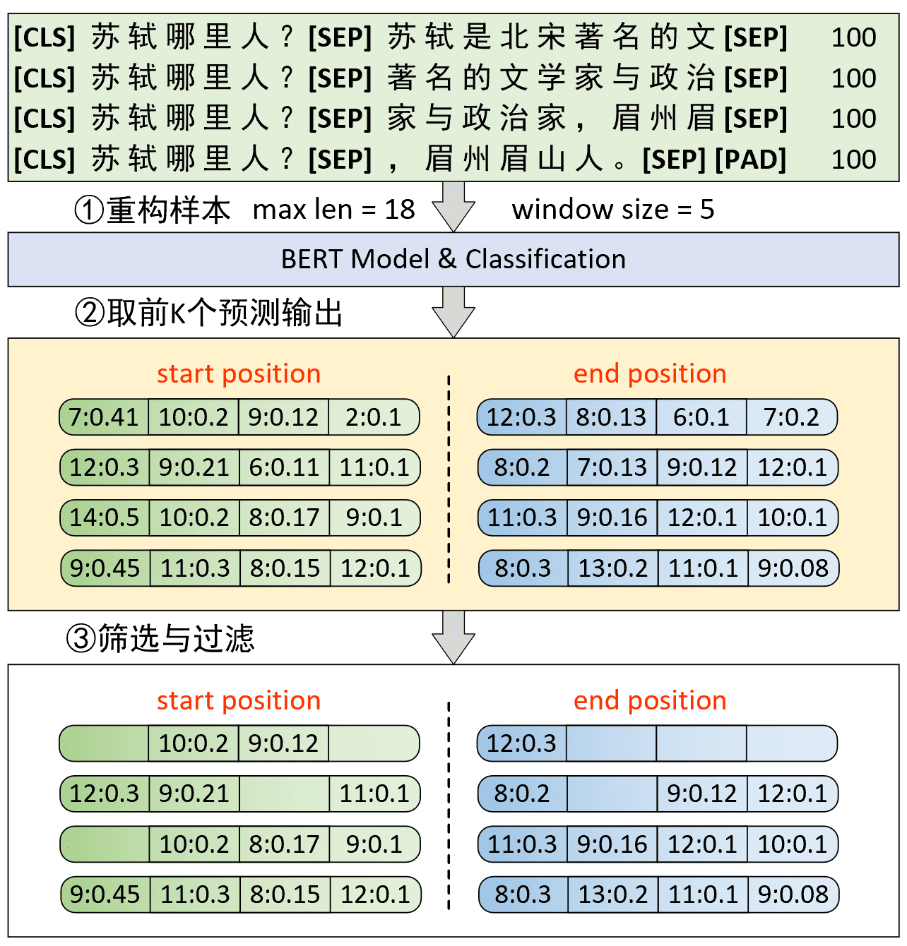
如图8-3所示,在推理过程中第①步要做的仍旧是需要根据指定最大长度和滑动窗口大小将原始样本进行滑动窗口处理。接着第②步便是根据BERT分类的输出取前K个概率值最大的结果。在图3中这里的K值为4,因此对于每个子样本来说其start position和end position分别都有4个候选结果。例如,第②步中第1行的 7:0.41,10:0.2,9:0.12,2:0.1 表示函数就是对于第1个子样本来说,start position为索引7的概率值为 0.41 ,其它同理。
这样对于每一个子样本来说,在分别得到start position和end position的K个候选值后便可以通过组合来得到更多的候选预测结果,然后再根据一些规则来选择最终原始样本对应的预测输出。
根据图8-3中样本重构后的结果可以看出:(1)最终的索引预测结果肯定是大于8的,因为答案只可能在上下文中出现;(2)在进行结果组合的过程中,起始索引肯定是小于等于结束索引的。因此,根据这两个条件在经过步骤③的处理后,便可以得到进一步的筛选结果。例如,对于第1个子样本来说,start position中7和2是不满足条件(1)的,所以可以直接去掉;同时,为了满足第(2)个条件所以在end position中8,6,7均需要去掉。
进一步,将第③步处理后的结果在每个子样本内部进行组合,并按照 start position 加 end position 值的大小进行排序,便可以得到如图 8-4 所示的结果。
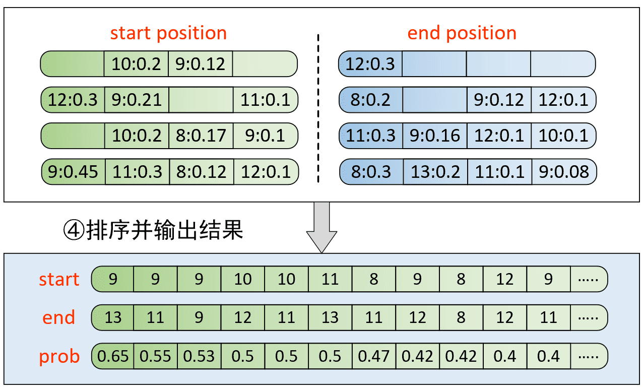
如图8-4所示表示根据概率和排序后的结果。例如第1列9,13,0.65的含义便是最终原始样本预测结果为9,13的概率值为0.65。因此,最终该原始样本对应的预测值便可以取9和13。
8.2.3 语料介绍#
由于没有找到类似的高质量中文数据集,所以在这里我们使用到的也是论文中所提到的SQuAD(The Stanford Question Answering Dataset 1.1 )数据集[19],即给定一个问题和描述需要模型从描述中找出答案的起止位置(找不到数据集的客官也可以找我们要)。
从第8.1节内容的介绍来看,在问题回答这个任务场景中模型的整体原理并不复杂,只不过需要通过滑动窗口来重构输入,所以后续我们在预处理数据集的时候还需要费点功夫。同时,SQuAD数据集本身的结构也略显复杂,所以这也相应加大了整个数据集构建的工作难度。如果不太想了解SQuAD数据集的构建流程也可以直接跳到对应预处理完成后的内容。下面我们就带着各位客官来一起梳理数据集的结构信息。
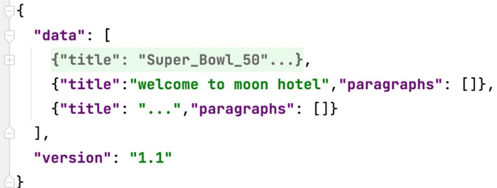
如图8-5所示便是数据集SQuAD1.1的结构形式。它整体由一个json格式的数据组成,其中的数据部分就在字段“data”中。可以看到data中存放的是一个列表,而列表中的每个元素可以看成是一篇文章,并以字典进行的存储。进一步,对于每一篇文章来说,其结构如图8-6所示。
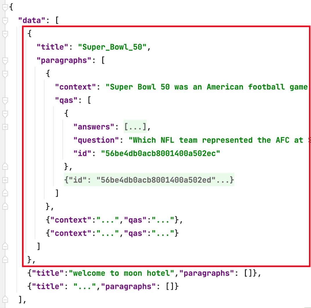
如图8-6所示,对于data中的每一篇文章来说,由“title”和“paragraphs”这两个字段组成。可以看到paragraphs是一个列表,其中的每一个元素为一个字典,可以看做是每一篇文章的其中一个段落,即后续需要使用到的上下文描述context。对于每一个段落来说,其包含有一段描述(“context”字段)和若干个问题与答案对(“qas”字段),其结构如图8-7所示。
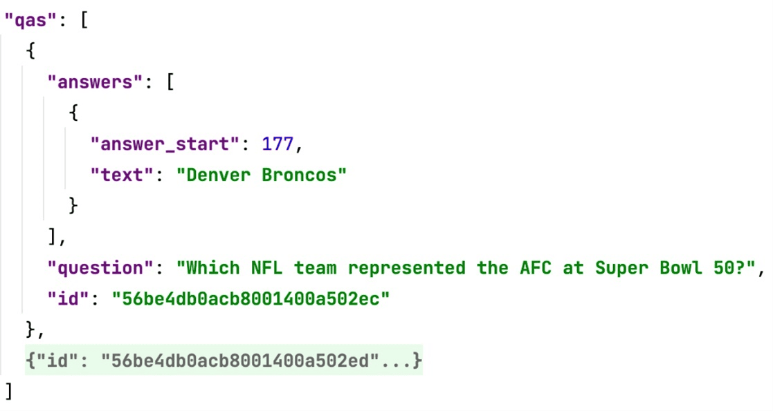
如图8-7所示,对于每个段落对应的问题组qas来说,其每一个元素都是答案(“answers”字段)、问题(“question”字段)和ID(“id”字段)的字典形式。同时,这里的“answer_start”只是答案在context中字符层面的索引,而不是每个单词在context中的位置,所以后面还需要进行转换。而我们所需要完成的便是从数据集中提取出对应的context、question、start pos、end pos以及id信息。
到此,对于数据集SQuAD1.1的基本信息就介绍完了。下面就开始来一步步介绍如何构建数据集。
8.2.4 数据集预览#
在正式介绍如何构建数据集之前我们同样先通过一张图来了解一下整个大致构建的流程。假如我们现在有两个样本构成了一个batch,那么其整个数据的处理过程则如图8-8所示。由于英文样例普遍较长画图不太方便,所以这里就以中文进行了示例,不过两者原理都一样。
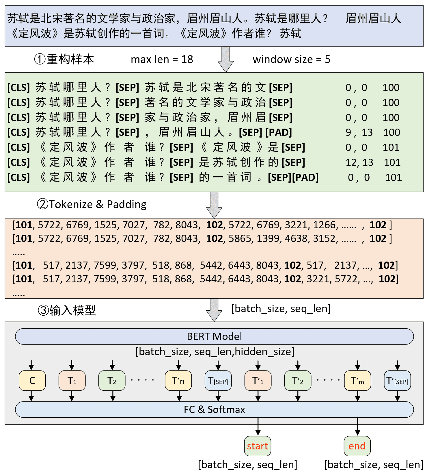
如图8-8所示,首先对于原始数据中的上下文按照指定的最大长度和滑动窗口大小进行滑动处理,然后再将问题同上下文拼接在一起构造成为一个序列并添加上对应的分类符[CLS]和分隔符[SEP],即图中的第①步重构样本。紧接着需要将第①步构造得到的序列转换得到Token id并进行padding处理,此时便得到了一个形状为[batch_size,seq_len]的2维矩阵,即图8中第②步处理完成后形状为[7,18]的结果。同时,在第②步中还要根据每个序列构造得到相应的attention_mask向量和token_types_ids向量(图中未画出),并且两者的形状也是[batch_size,seq_len]。
最后,将第②步处理后的结果输入到BERT模型中,在经过BERT特征提取后将会得到一个形状为[batch_size,seq_len,hidden_size]的3维矩阵,最后再乘上一个形状为[hidden_size,2]的矩阵并变形成[batch_size,seq_len,2]的形状,即是对每个Token进行分类。
8.2.5 数据集构造#
在说完数据集构造的整理思路后,下面我们就来正式编码实现整个数据集的构造过程。同样,对于数据预处理部分我们可以继续继承之前文本分类处理的这个类LoadSingleSentenceClassificationDataset,然后再稍微修改其中的部分方法即可。同时,由于在前几个示例中已经就tokenize和词表构建等内容做了详细的介绍,所以这部分内容就不再赘述。
(1) 规整化原始数据
以下数据预处理代码主要参考自 https://github.com/google-research/bert 中的 run_squad.py 脚本。
第1步:格式化文本
从图8-7可以看出,SQuAD原始数据集给出的每个问题的答案并不是标准的start pos和end pos,因此我们需要自己编写一个函数来根据answer_start和text字段来获得答案在原始上下文中的start pos和end pos(单词级别),实现代码如下所示:
 1     @staticmethod
 2     def get_format_text_and_word_offset(text):
 3
 4         def is_whitespace(c):
 5             if c == " " or c == "\t" or c == "\r" or c == "\n" or ord(c) == 0x202F:
 6                 return True
 7             return False
 8
 9         doc_tokens = []
10         char_to_word_offset = []
11         prev_is_whitespace = True
12         # 以下这个for循环的作用就是将原始context中的内容进行格式化
13         for c in text:  # 遍历paragraph中的每个字符
14             if is_whitespace(c):  # 判断当前字符是否为空格(各类空格)
15                 prev_is_whitespace = True
16             else:
17                 if prev_is_whitespace:  # 如果前一个字符是空格
18                     doc_tokens.append(c)
19                 else:
20                     doc_tokens[-1] += c  # 在list的最后一个元素中继续追加字符
21                 prev_is_whitespace = False
22             char_to_word_offset.append(len(doc_tokens) - 1)
23         return doc_tokens, char_to_word_offset
如上代码所示便是该函数的整体实现,其主要思路为:①第12~13行,依次遍历原始字符串中的每一个字符,然后判断其前一个字符是否为空格;②第15~17行,如果前一个字符是空格那么表示当前字符是一个新单词的开始,因此可以将前面的多个字符append到list中作为一个单词;③第18~19行,如果不是空格那么表示当前的字符仍旧属于上一个单词的一部分,因此将当前字符继续追加到上一个单词的后面;④同时,第21行用来记录当前当前字符所属单词的索引偏移量,这样根据 answer_start字段来取 char_to_word_offset 中对应位置的值便得到了问题答案在上下文中的起始位置。
例如对于如下文本来说:
1 text = "Architecturally, the school has a Catholic character. "函数 get_format_text_and_word_offset() 返回的结果便是:
1 doc_tokens = ['Architecturally,', 'the', 'school', 'has', 'a', 'Catholic',
2               'character.'],
3 char_to_word_offset = [0, 0, 0, 0, 0, 0, 0, 0, 0, 0, 0, 0, 0, 0, 0, 0, 0, 1,
4                        1, 1, 1, 2, 2, 2, 2, 2, 2, 2, 3, 3, 3, 3, 4, 4, 5, 5,
5                        5, 5, 5, 5, 5, 5, 5, 6, 6, 6, 6, 6, 6, 6, 6, 6, 6, 6]
例如单词school在原始text中的起始位置为21(字符级别),那么根据 char_to_word_offset[21] 便可以返回的到school在原始文本中的位置为2。
此时,细心的客官可能发现,返回的doc_tokens中有的单词里还包含有符号,并且很多单词在经过tokenize后还会被拆分成多个部分,因此这里只是暂时得到一个初步的起始位置,后续还会进行修正。
第2步:读取数据
根据图8-5到图8-7的展示,下面我们需要定义一个函数来对原始数据进行读取得到每个样本原始的字符串形式。
 1 class LoadSQuADQuestionAnsweringDataset(LoadSingleSentenceClassificationDataset):
 2
 3     def __init__(self, doc_stride=64,
 4                  max_query_length=64,
 5                  n_best_size=20,
 6                  max_answer_length=30,
 7                  kwargs):
 8         super(LoadSQuADQuestionAnsweringDataset, self).__init__(kwargs)
 9         self.doc_stride = doc_stride
10         self.max_query_length = max_query_length
11         self.n_best_size = n_best_size
12         self.max_answer_length = max_answer_length
13
14     def preprocessing(self, filepath, is_training=True):
15         with open(filepath, 'r') as f:
16             raw_data = json.loads(f.read())
17             data = raw_data['data']
18         examples = []
19         ……
在上述代码中,首先定义了类 LoadSQuADQuestionAnsweringDataset 并继承自之前的 LoadSingleSentenceClassificationDataset 类;第9~q行分别表示滑动窗口的长度,以及问题的最大长度;第14~19行便是定义 preprocessing 函数用来对原始json数据进行读取,其中第17行返回的便是整个json格式的原始数据。
下面开始遍历json数据中的每个 paragraph:
 1     def preprocessing(self, filepath, is_training=True):
 2         # 接上面代码
 3         for i in tqdm(range(len(data)), ncols=80, desc="正在遍历每一个段落"):
 4             paragraphs = data[i]['paragraphs']
 5             for j in range(len(paragraphs)):
 6                 context = paragraphs[j]['context']
 7                 context_tokens, word_offset = self.get_format_text_and_word_offset(context)
 8                 qas = paragraphs[j]['qas']
 9                 for k in range(len(qas)):
10                     question_text = qas[k]['question']
11                     qas_id = qas[k]['id']
12                     if is_training:
13                         answer_offset = qas[k]['answers'][0]['answer_start']
14                         orig_answer_text = qas[k]['answers'][0]['text']
15                         answer_length = len(orig_answer_text)
16                         start_position = word_offset[answer_offset]
17                         end_position = word_offset[answer_offset + answer_length - 1]
18                         actual_text = " ".join(context_tokens
19                                       [start_position:(end_position + 1)])
20                         cleaned_answer_text = " ".join(orig_answer_text.strip().split())
21                         if actual_text.find(cleaned_answer_text) == -1:
22                             logging.warning("Could not find answer: '%s' vs. '%s'", actual_text, cleaned_answer_text)
23                             continue
24                     else:
25                         start_position = None
26                         end_position = None
27                         orig_answer_text = None
28                     examples.append([qas_id, question_text, orig_answer_text, " ".join(context_tokens), start_position, end_position])
29         return examples
在上述代码中,第3~4行用来遍历原始数据中的每一篇文章;第5~8行用来遍历每一篇文章中的每个paragraph,并取相应的上下文context和问题-答案对;第9~11行是用来遍历取每个paragraph中对应的多个问题和问题id;第12~23行表示,如果当前处理的是训练集,那么再取问题对应的 answer_offset、orig_answer_text 并以此获取原始答案对应的起始位置 start_position 和结束位置 end_position ;第18~22行则是判断真实答案和根据起止位置从context中截取的答案是否相同,不同则跳过该条样本;第25~27行是用来处理验证集或测试集。
最后,该函数将会返回一个2维列表,内层列表中的各个元素分别为:
1 ['问题ID','原始问题文本','答案文本','context文本','答案在context中的开始位置', '答案在context中的结束位置']例如:
1 [['5733be284776f41900661182', 'To whom did the Virgin Mary allegedly appear in .... France?', 'Saint Bernadette Soubirous', 'Architecturally, the school has a Catholic character......', 90, 92],
2  ['5733be284776f4190066117f', ....]]
第3步:修正起止位置
在上面我们提到,此时得到的起止位置会因为不同的tokenize而产生变化,因此需要进一步进行修正。同时,原始文本中”(1895-1943)“这类形式的字符串也会被认为是一个单词,但是在tokenize后也会发生变化,所以需要一同进行处理。实现代码如下所示:
 1     @staticmethod
 2     def improve_answer_span(context_tokens,
 3                             answer_tokens,
 4                             start_position,
 5                             end_position):
 6         new_end = None
 7         for i in range(start_position, len(context_tokens)):
 8             if context_tokens[i] != answer_tokens[0]:
 9                 continue
10             for j in range(len(answer_tokens)):
11                 if answer_tokens[j] != context_tokens[i + j]:
12                     break
13                 new_end = i + j
14             if new_end - i + 1 == len(answer_tokens):
15                 return i, new_end
16 return start_position, end_position在上述代码中,context_tokens 为已经 tokenize 后的原始上下文;answer_tokens 为原始答案文本经过 tokenize 后的结果,例如:
1 context = "Virgin mary reputedly appeared to Saint Bernadette Soubirous in 1858"
2 answer_text = "Saint Bernadette Soubirous"
3 start_position = 5
4 end_position = 7
5 context_tokens: ['virgin', 'mary', 'reputed', '##ly', 'appeared', 'to',
6 'saint','bern', '##ade', '##tte', 'so', '##ub', '##iro', '##us', 'in','1858']
7 answer_tokens: ['saint', 'bern', '##ade', '##tte','so','##ub','##iro', '##us'
则其返回后新的起止位置为[6,13]。
这段代码的主要思路是以原始起始位置开始,依次将后续的每个片段同answer_tokens进行对比,如果context_tokens中的子片段等同于answer_tokens,那么就返回新的起止位置;否则还是返回传入的起止位置。
同样,对于下面的示例:
1 context = "The leader was John Smith (1895-1943).
2 answer_test = "1985"
3 answer_tokens: ["1895"]
4 start_position: 5
5 end_position: 5
6 context_tokens: ['the', 'leader', 'was', 'john', 'smith', '(', '1895', '-', '1943', ')', '.']
返回新的起止位置便为[6,6]。
(2) 重构输入样本
在通过预处理函数 preprocessing() 后,我们便可以来进一步地采用滑动窗口方式来构造模型的输入。由于这部分代码稍微有点长,所以下面就分块进行介绍。
 1     @cache
 2     def data_process(self, filepath, is_training=False, postfix='cache'):
 3         logging.info(f"## 使用窗口滑动滑动,doc_stride = {self.doc_stride}")
 4         examples = self.preprocessing(filepath, is_training)
 5         all_data = []
 6         example_id, feature_id = 0, 1000000000
 7         for example in tqdm(examples,ncols=80,desc="正在遍历每个问题(样本)"):
 8             question_tokens = self.tokenizer(example[1])
 9             if len(question_tokens) > self.max_query_length:# 问题过长进行截取
10                 question_tokens = question_tokens[:self.max_query_length]
11             question_ids = [self.vocab[token] for token in question_tokens]
12             question_ids = [self.CLS_IDX] + question_ids + [self.SEP_IDX]
13             context_tokens = self.tokenizer(example[3])
14             context_ids = [self.vocab[token] for token in context_tokens]
15             logging.debug(f"<<<<<<<<  进入新的example  >>>>>>>>>")
16             logging.debug(f"## 正在预处理数据 {__name__} is_training = {is_training}")
17             logging.debug(f"## 问题 id: {example[0]}")
18             logging.debug(f"## 原始问题 text: {example[1]}")
19             logging.debug(f"## 原始描述 text: {example[3]}")
20             start_position, end_position, answer_text = -1, -1, None
21             if is_training:
22                 start_position, end_position = example[4], example[5]
23                 answer_text = example[2]
24                 answer_tokens = self.tokenizer(answer_text)
25                 start_position, end_position = self.improve_answer_span(
26                    context_tokens,answer_tokens,start_position,end_position)
27             rest_len = self.max_sen_len - len(question_ids) - 1
28             context_ids_len = len(context_ids)
29             logging.debug(f"## 上下文长度为:{context_ids_len},剩余长度rest_len 为:{rest_len}")
在上述代码中,第1行@cache的作用是将 data_process() 处理后的结果进行缓存,以方便下次直接从本地载入节约时间,具体原理可以参见文章 [27];第7行则是开始遍历 preprocessing() 函数返回的每一条原始数据;第8~14行则是取对应我们后续所需要的成分;第21~26行则是用来获取得到训练集中 start_position、 end_position以及 answer_text ;第27~28行是用来计算context的长度判读是否需要进行滑动窗口处理。
以下代码则是滑动窗口处理部分:
 1             if context_ids_len > rest_len: # 长度超过max_sen_len,需要进行滑动窗口
 2                 logging.debug(f"## 进入滑动窗口 …… ")
 3                 s_idx, e_idx = 0, rest_len
 4                 while True:
 5                     tmp_context_ids = context_ids[s_idx:e_idx]
 6                     tmp_context_tokens = [self.vocab.itos[item] for item
 7                                                      in tmp_context_ids]
 8                     input_ids = torch.tensor(question_ids +
 9                                         tmp_context_ids + [self.SEP_IDX])
10                     input_tokens = ['[CLS]'] + question_tokens +
11                                 ['[SEP]'] +tmp_context_tokens + ['[SEP]']
12                     seg = [0]  len(question_ids) + [1]  (len(input_ids)
13                                                      - len(question_ids))
14                     seg = torch.tensor(seg)
15                     if is_training:
16                         new_start_position, new_end_position = 0, 0
17                         if start_position >=s_idx and end_position <= e_idx:
18                             logging.debug(f"## 滑动窗口中存在答案 -----> ")
19                             new_start_position = start_position - s_idx
20                             new_end_position = new_start_position +
21                                           (end_position - start_position)
22                             new_start_position += len(question_ids)
23                             new_end_position += len(question_ids)
24                         all_data.append([example_id, feature_id, input_ids,
25                                   seg, new_start_position,new_end_position,
26                                     answer_text, example[0], input_tokens])
27                         logging.debug(f"## start pos:{new_start_position}")
28                         logging.debug(f"## end pos:{new_end_position}")
29                     else:
30                         all_data.append([example_id, feature_id, input_ids,
31                               seg, start_position,end_position, answer_text,
32                               example[0], input_tokens])
33                         logging.debug(f"## start pos:{start_position}")
34                         logging.debug(f"## end pos:{end_position}")
35                     token_to_orig_map = self.get_token_to_orig_map(input_tokens,
36                                    example[3], self.tokenizer)
37                     all_data[-1].append(token_to_orig_map)
38                     feature_id += 1
39                     if e_idx >= context_ids_len:
40                         break
41                     s_idx += self.doc_stride
42                     e_idx += self.doc_stride
在上述代码中,第4代码开始便是进入滑动窗口循环处理中;第5~14行则是构造得到相应的所需部分,包括 input ids、input tokens和segment ids等;第15~32行是分别取训练和预测时输入序列对应答案所在的索引位置,并同其余部分形成一个原始样本存入 all_data 当中;第32~36行则是返回得 input_tokens 中每个Token在原始单词中所对应的位置索引,这一结果将会在最后推理过程中得到最后预测结果时用到。
例如现在有如下Token:
1 input_tokens = ['[CLS]', 'to', 'whom', 'did', 'the', 'virgin', '[SEP]',
2 'architectural', '##ly', ',', 'the', 'school', 'has', 'a', 'catholic',
3 'character', '.', '[SEP']
那么上下文Token在原始上下文中的索引映射表则为:
1 origin_context = "Architecturally, the Architecturally, test, Architecturally,  the school has a Catholic character. Welcome moon hotel"
2 orig_map = {7: 4, 8: 4, 9: 4, 10: 5, 11: 6, 12: 7, 13: 8, 14: 9,15:10,16: 10}
其含义表示,input_tokens[7]为 origin_context 中的第4个单词 Architecturally,同理 input_tokens[10] 为 origin_context 中的第5个单词 the。
以下代码则是非滑动窗口处理部分
 1            else:
 2                 input_ids = torch.tensor(question_ids + context_ids + [self.SEP_IDX])
 3                 input_tokens = ['[CLS]'] + question_tokens + ['[SEP]'] + context_tokens + ['[SEP]']
 4                 seg = [0]  len(question_ids) + [1]  (len(input_ids) - len(question_ids))
 5                 seg = torch.tensor(seg)
 6                 if is_training:
 7                     start_position += (len(question_ids))
 8                     end_position += (len(question_ids))
 9                 token_to_orig_map = self.get_token_to_orig_map(input_tokens, example[3], self.tokenizer)
10                 all_data.append([example_id, feature_id, input_ids, seg, start_position,
11                                  end_position, answer_text, example[0], input_tokens, token_to_orig_map])
12                 logging.debug(f"## input_tokens: {input_tokens}")
13                 logging.debug(f"## input_ids:{input_ids.tolist()}")
14                 logging.debug(f"## segment ids:{seg.tolist()}")
15                 logging.debug(f"## orig_map:{token_to_orig_map}")
16                 logging.debug("======================\n")
17                 feature_id += 1
18             example_id += 1
19         data = {'all_data': all_data, 'max_len': self.max_sen_len, 'examples': examples}
20         return data
其中 all_data 中的每个元素分别为:原始样本id、训练特征id、input_ids、seg、开始位置、结束位置、答案文本、问题id、input_tokens和ori_map。
(3) 构造DataLoader
在完成前面两部分内容后,只需要在构造每个batch时对输入序列进行padding并返回的相应的 DataLoader 整个数据集就算是构造完成了。为此,首先需要定义一个函数来构造每一个batch,代码如下:
 1     def generate_batch(self, data_batch):
 2         batch_input, batch_seg, batch_label, batch_qid = [], [], [], []
 3         batch_example_id, batch_feature_id, batch_map = [], [], []
 4         for item in data_batch:
 5             # item: [原始样本Id,训练特征id,input_ids,seg,开始,
 6             #        结束,答案文本,问题id,input_tokens,ori_map]
 7             batch_example_id.append(item[0])  # 原始样本Id
 8             batch_feature_id.append(item[1])  # 训练特征id
 9             batch_input.append(item[2])  # input_ids
10             batch_seg.append(item[3])  # seg
11             batch_label.append([item[4], item[5]])  # 开始, 结束
12             batch_qid.append(item[7])  # 问题id
13             batch_map.append(item[9])  # ori_map
14
15         batch_input = pad_sequence(batch_input,  # [batch_size,max_len]
16                       padding_value=self.PAD_IDX,batch_first=False,
17                       max_len=self.max_sen_len)  # [max_len,batch_size]
18         batch_seg = pad_sequence(batch_seg,  # [batch_size,max_len]
19                       padding_value=self.PAD_IDX,batch_first=False,
20                       max_len=self.max_sen_len)  # [max_len, batch_size]
21         batch_label = torch.tensor(batch_label, dtype=torch.long)
22         # [max_len,batch_size] , [max_len, batch_size] , [batch_size,2], [batch_size,], [batch_size,]
23         return batch_input, batch_seg, batch_label, batch_qid, batch_example_id, batch_feature_id, batch_map
在上述代码中,第1行中的 data_batch 便是 data_process() 处理后返回的all_data;第4~13行便是构造每个 batch 中所包含的向量;第15~21行则是根据指定的参数 max_len 来进行padding处理(关于 pad_sequence 函数的详细介绍见「第4.2.4节 BERT 文本分类实战教程:从 [CLS] 微调到 38 万今日头条 15 类新闻分类」 中的内容讲解);第23行是用来返回每个batch处理后的结果
进一步,构造得到数据集对应的DataLoader,代码如下:
 1     def load_train_val_test_data(self, train_file_path=None,
 2                                  val_file_path=None,
 3                                  test_file_path=None,
 4                                  only_test=True):
 5         doc_stride = str(self.doc_stride)
 6         max_sen_len = str(self.max_sen_len)
 7         max_query_length = str(self.max_query_length)
 8         postfix = doc_stride + '_' + max_sen_len + '_' + max_query_length
 9         data = self.data_process(filepath=test_file_path,
10                                  is_training=False,postfix=postfix)
11         test_data, examples = data['all_data'], data['examples']
12         test_iter = DataLoader(test_data, batch_size=self.batch_size,
13                     shuffle=False,collate_fn=self.generate_batch)
14         if only_test:
15             return test_iter, examples
16
17         data = self.data_process(filepath=train_file_path,
18                         is_training=True,postfix=postfix)
19         train_data, max_sen_len = data['all_data'], data['max_len']
20         _, val_data = train_test_split(train_data, test_size=0.3, random_state=2021)
21         if self.max_sen_len == 'same':
22             self.max_sen_len = max_sen_len
23         train_iter = DataLoader(train_data, batch_size=self.batch_size,
24             shuffle=self.is_sample_shuffle, collate_fn=self.generate_batch)
25         val_iter = DataLoader(val_data, batch_size=self.batch_size,
26                               shuffle=False, collate_fn=self.generate_batch)
27         logging.info(f"## 成功返回训练集样本({len(train_iter.dataset)})个、"
28                      f"开发集样本({len(val_iter.dataset)})个"
29                      f"测试集样本({len(test_iter.dataset)})个.")
30         return train_iter, test_iter, val_iter
在上述代码中,第5~8行则是根据对应的超参数来构造一个数据预处理结果缓存的名称;第9~15行便是用来构造得到对应测试集的 DataLoader ;在第20行中,我们将原始的训练集又划分成了两个部分,并在第23~26行中分别返回了两者对应的 DataLoader 。
同时,这里特别需要注意的一点是,为了方便后续对预测结果进行处理,我们直接固定了验证集和测试集中每个样本的顺序,即 shuffle=False 。因为当 shuffle 为 True 时,每次通过 for 循环遍历 data_iter 时样本的顺序都不一样。
到此,对于整个SQuAD1.1版数据集的构建流程就介绍了。
(4) 使用示例
在完成上述3个步骤之后,可以通过如下代码进行数据集的载入:
 1 from utils.data_helpers import LoadSQuADQuestionAnsweringDataset
 2 from transformers import BertTokenizer
 3 from Tasks.TaskForSQuADQuestionAnswering import ModelConfig
 4
 5 if __name__ == '__main__':
 6     config = ModelConfig()
 7     tokenizer = BertTokenizer.from_pretrained(config.pretrained_model_dir)
 8     data_loader = LoadSQuADQuestionAnsweringDataset(
 9                   vocab_path=config.vocab_path,
10                   tokenizer=tokenizer.tokenize,batch_size=5,max_sen_len=120,
11                   max_position_embeddings=512,pad_index=0,
12                   is_sample_shuffle=False,
13                   doc_stride=8,max_query_length=5)
14
15     train_iter, test_iter, val_iter = data_loader. \
16         load_train_val_test_data(test_file_path=config.test_file_path,
17                                  train_file_path=config.train_file_path,
18                                  only_test=False)
19     for b_input, b_seg, b_label, b_qid, b_example_id, b_feature_id, b_map in train_iter:
20         print("=====================>")
21         print(f"intput_ids shape: {b_input.shape}") # [max_len, batch_size]
22         print(f"token_type_ids shape: {b_seg.shape}")# [max_len, batch_size]
23         print(b_seg.transpose(0, 1).tolist())
24         print(b_label)  # [batch_size,2]
25         print(b_map)  # [batch_size]
26         for i in range(b_input.size(-1)):
27             sample = b_input.transpose(0, 1)[i]
28             start_pos, end_pos = b_label[i][0], b_label[i][1]
29             strs = [data_loader.vocab.itos[s] for s in sample]  # 原始tokens
30             answer = " ".join(strs[start_pos:(end_pos+1)]).replace(" ##","")
31             strs = " ".join(strs).replace(" ##", "").split('[SEP]')
32             question, context = strs[0], strs[1]
33             print(f"问题ID:{b_qid[i]}")
34             print(f"问题:{question}")
35             print(f"正确答案:{answer}")
36             print(f"答案起止:{start_pos, end_pos}")
37             print(f"example ID:{b_example_id[i]}")
38             print(f"feature ID:{b_feature_id[i]}")
在上述代码中,第15~18行便是返回训练集、验证集和测试集对应的DataLoader;第19~25行是用来遍历训练集中每个batch的数据;第27~38行是遍历一个batch中的每个样本,并转换为对应的文本形式。
最后,上述代码输入结果将类似如下所示:
 1 -INFO: 导入配置~/BertWithPretrained/bert_base_uncased_english/config.json
 2 -INFO: ### 将当前配置打印到日志文件中
 3 -INFO: ### project_dir = ~/BertWithPretrained
 4 -INFO: ### dataset_dir = ~/BertWithPretrained/data/SQuAD
 5 -INFO: ### train_file_path = ~/BertWithPretrained/data/SQuAD/train-v1.1.json
 6 ......
 7 -INFO: ### model_save_path = ~/BertWithPretrained/cache/model.pt
 8 -INFO: ### n_best_size = 10
 9 -INFO: ### max_answer_len = 30
10 ......
11 -INFO: 缓存~/BertWithPretrained/data/SQuAD/dev-v1_8_120_5.pt 不存在,重新处理!
12 -INFO: ## 使用窗口滑动滑动,doc_stride = 8
13 正在遍历每一个段落: 100%|██████████| 48/48 [00:00<00:00, 60.80it/s]
14 正在遍历每个问题(样本):   0%|                  | 0/10570 [00:00<?, ?it/s]
15 -DEBUG: <<<<<<<<  进入新的example  >>>>>>>>>
16 -DEBUG: ## 正在预处理数据 utils.data_helpers is_training = False
17 -DEBUG: ## 问题 id: 56be4db0acb8001400a502ec
18 -DEBUG: ## 原始问题 text:Which NFL team represented the AFC at Super Bowl 50?
19 -DEBUG: ## 原始描述 text: Super Bowl 50 was an American football game to determine the champion of the National Football League (NFL) for the 2015 season. The American Football Conference (AFC) champion  ......
20 -DEBUG: ## 上下文长度为:157, 剩余长度 rest_len 为 : 112
21 -DEBUG: ## 滑动窗口范围:(0, 112),example_id: 0, feature_id: 1000000000
22 -DEBUG: ## start pos:-1 end pos:-1 end pos:-1 end pos:-1
23 -DEBUG: ## input_tokens: ['[CLS]', 'which', 'nfl', 'team', 'represented', 'the', '[SEP]', 'super', 'bowl', '50', 'was', 'an', 'american', 'football', 'game', 'to', 'determine', 'the', 'champion', ......, '[SEP]']
24 -DEBUG: ## input_ids:[101, 2029, 5088, 2136, 3421, 1996, 102, 3565, 4605, 2753, 2001, 2019, 2137, 2374, 2208, 2000, 5646, 1996, 3410, 1997, 1996, 2120, 2374, 2223, 1006, 5088, 1007, 2005, 1996, 2325, ......, 102]
25 -DEBUG: ## segment ids:[0, 0, 0, 0, 0, 0, 0, 1, 1, 1, 1, 1, 1, 1, 1, 1, 1, 1, 1, 1, 1, 1, 1, 1, 1, 1,  ......1]
26 -DEBUG: ## orig_map:{7: 0, 8: 1, 9: 2, 10: 3, 11: 4, 12: 5, 13: 6, 14: 7, 15: 8, 16: 9, 17: 10, 18: 11, 19: 12, 20: 13, 21: 14, 22: 15, 23: 16, 24: 17, 25: 17, 26: 17, 27: 18, ......}
27 -DEBUG: ======================
28 问题ID:5733bf84d058e614000b61c1
29 问题:[CLS] in what year did the
30 正确答案:1987
31 答案起止:(tensor(60), tensor(60))
32 example ID:9
33 feature ID:1000000125
34 问题ID:5733bf84d058e614000b61c1
35 问题:[CLS] in what year did the
36 正确答案:1987
……
到此,对于整个数据集的介绍就完了。如果是正在研究这类问题回答模型的客官,强烈建议你结合本文一行一行地去阅读本项目中的原始代码,你一定会受益匪浅。
下面我们开始继续介绍问题回答模型的实现部分。
8.3 问答任务#
8.3.1 前向传播#
正如第8.1节内容所介绍,我们只需要在原始BERT模型的基础上取最后一层的输出结果,然后再加一个分类层即可。因此这部分代码相对来说也比较容易理解。
如图2-4所示,在 BertForMultipleChoice.py 模块中,首先需要定义一个类以及相应的初始化函数,代码如下:
 1 from ..BasicBert.Bert import BertModel
 2 import torch.nn as nn
 3
 4 class BertForQuestionAnswering(nn.Module):
 5
 6     def __init__(self, config, bert_pretrained_model_dir=None):
 7         super(BertForQuestionAnswering, self).__init__()
 8         if bert_pretrained_model_dir is not None:
 9             self.bert = BertModel.from_pretrained(config, bert_pretrained_model_dir)
10         else:
11             self.bert = BertModel(config)
12         self.qa_outputs = nn.Linear(config.hidden_size, 2)
在上述代码中,第8~11行便是根据相应的条件返回一个BERT模型,第12行则是定义了一个分类层。
然后再是定义完成整个前向传播过程,代码如下:
 1     def forward(self, input_ids,attention_mask=None,
 2                 token_type_ids=None,position_ids=None,
 3                 start_positions=None,end_positions=None):
 4         _, all_encoder_outputs = self.bert(
 5             input_ids=input_ids,attention_mask=attention_mask,
 6             token_type_ids=token_type_ids,position_ids=position_ids)
 7         sequence_output = all_encoder_outputs[-1]  # 取Bert最后一层的输出
 8         # sequence_output: [src_len, batch_size, hidden_size]
 9         logits = self.qa_outputs(sequence_output)  # [src_len, batch_size,2]
10         start_logits, end_logits = logits.split(1, dim=-1)
11         # [src_len,batch_size,1]  [src_len,batch_size,1]
12         start_logits = start_logits.squeeze(-1).transpose(0, 1)
13         end_logits = end_logits.squeeze(-1).transpose(0, 1)
14         if start_positions is not None and end_positions is not None:
15             ignored_index = start_logits.size(1)  # 取输入序列的长度
16             start_positions.clamp_(0, ignored_index)
17             end_positions.clamp_(0, ignored_index)
18             loss_fct = nn.CrossEntropyLoss(ignore_index=ignored_index)
19             start_loss = loss_fct(start_logits, start_positions)
20             end_loss = loss_fct(end_logits, end_positions)
21             return (start_loss + end_loss) / 2, start_logits, end_logits
22         else:
23             return start_logits, end_logits  # [batch_size,src_len]
在上述代码中,第4~7行便是根据输入返回原始BERT模型的输出结果,需要注意的是这里要取BERT输出整个最后1层的输出结果,而不是像之前一样只取最后1层第1个位置[CLS]对应的向量。第9行便是分类层的输出结果,形状为[src_len, batch_size,2]。第10~13行则是得到对应的 start_logits 和 end_logits ,两者的形状均是[batch_size,src_len]。第14~23行则是根据是否有标签返回对应的损失或者logits值;第15~17行是用来处理当给定的 start_positions 和 end_positions 在[0,max_len]这个范围之外时,强制将其改为0或 max_len ;例如某个样本的起始位置为520,而序列最大长度为512(即此时 ignore_index=512 ),那么 clamp_() 方法便会将520改变成512,当然根据前面我们的数据处理流程来最后生成的数据集并不存在这样的情况,这里只是以防万一。在第18行中,之所以要将 ignored_index 作为损失计算时的忽略值,是因为这些位置并不能算是模型预测错误的(只能看做是没有预测),而是答案超出了范围所以需要忽略掉这些情况.最后,第19~20行是分别计算。
到此,对于问题回答任务的模型定义就介绍完了,可以看出这一过程也并不复杂。我们这里依旧建议各位客官在阅读代码时能够带着对应维度进行理解,以便对每一步变换有着清晰的认识。
8.3.2 模型训练#
首先,如图2-5所示在 Tasks 目录下新建一个名为 TaskForSQuADQuestionAnswering.py 的模块,然后定义一个 ModelConfig 类来对分类模型中的超参数以及其它变量进行管理。部分代码如下所示:
1 class ModelConfig:
 2     def __init__(self):
 3         self.project_dir = os.path.dirname(os.path.dirname(os.path.abspath(__file__)))
 4         self.dataset_dir = os.path.join(self.project_dir, 'data', 'SQuAD')
 5         self.vocab_path=os.path.join(self.pretrained_model_dir, 'vocab.txt')
 6         self.train_file_path=os.path.join(self.dataset_dir,'train-1.1.json')
 7         self.test_file_path =os.path.join(self.dataset_dir, 'dev-v1.1.json')
 8         self.model_save_dir = os.path.join(self.project_dir, 'cache')
 9         self.logs_save_dir = os.path.join(self.project_dir, 'logs')
10         self.model_save_path = os.path.join(self.model_save_dir, 'model.pt')
11         self.n_best_size = 10
12         self.max_answer_len = 30
13         self.is_sample_shuffle = True
14         self.use_torch_multi_head = False
15         self.max_sen_len = 384
16         self.max_query_len = 64  #
17         self.doc_stride = 128
18         self.epochs = 2
19         self.model_val_per_epoch = 1
20         logger_init(log_file_name='qa', log_level=logging.D
21                     log_dir=self.logs_save_dir)
在上述代码中,第11行是对预测出的答案进行后处理时,选取的候选答案数量,这个将在下一小节中进行介绍。第12行是在对候选进行筛选时,对答案最大长度的限制。第13行表示是否对训练集进行打乱。第14行表示是否使用PyTorch中的 multihead 实现,如果为 False 则使用项目 MyTransformer.py 中的多头注意力实现,如果是 True 则会使用 torch.nn.MultiheadAttention 中的多头注意力实现。第15行是最大句子长度,即 [CLS] + question ids + [SEP] + context ids + [SEP] 的长度。第16行是问题的最大长度,超过长度则进行截取。第17行是滑动窗口一次滑动的长度。
紧接着,我们便可以定义函数 train() 来完成模型的训练:
 1 def train(config):
 2     model = BertForQuestionAnswering(config,config.pretrained_model_dir)
 3     if os.path.exists(config.model_save_path):
 4         loaded_paras = torch.load(config.model_save_path)
 5         model.load_state_dict(loaded_paras)
 6         logging.info("## 成功载入已有模型,进行追加训练......")
 7     tokenize = BertTokenizer.from_pretrained(config.pretrained_model_dir)
 8     data_loader = LoadSQuADQuestionAnsweringDataset(
 9                 vocab_path=config.vocab_path,
10                 tokenizer=tokenize.tokenize,batch_size=config.batch_size,
11                 max_sen_len=config.max_sen_len,
12                 max_query_length=config.max_query_len,
13                 max_position_embeddings=config.max_position_embeddings,
14                 pad_index=config.pad_token_id,
15                 is_sample_shuffle=config.is_sample_shuffle,
16                 doc_stride=config.doc_stride)
17     train_iter, test_iter, val_iter = \
18         data_loader.load_train_val_test_data(
19                    train_file_path=config.train_file_path,
20                    test_file_path=config.test_file_path,only_test=False)
21     lr_scheduler = get_scheduler(name='linear',optimizer=optimizer,
22                     num_warmup_steps=int(len(train_iter)  0),
23                     num_training_steps=int(config.epochs  len(train_iter)))
24     max_acc = 0
25     for epoch in range(config.epochs):
26         for idx, (batch_input, batch_seg, batch_label, _, _, _, _) in enumerate(train_iter):
27             padding_mask=(batch_input== data_loader.PAD_IDX).transpose(0, 1)
28             loss, start_logits, end_logits = model(input_ids=batch_input,
29                     attention_mask=padding_mask, token_type_ids=batch_seg,
30                     position_ids=None, start_positions=batch_label[:, 0],
31                     end_positions=batch_label[:, 1])
32             lr_scheduler.step()
33             ......
34             if idx % 100 == 0:
35                 y_pred = [start_logits.argmax(1), end_logits.argmax(1)]
36                 y_true = [batch_label[:, 0], batch_label[:, 1]]
37                 show_result(batch_input,data_loader.vocab.itos,y_predy_true)
38         if (epoch + 1) % config.model_val_per_epoch == 0:
39             acc = evaluate(val_iter,model,config.device,data_loader.PAD_IDX,False)
40             logging.info(f"## Acc on val:{round(acc, 4)} max :{max_acc}")
在上述代码中,第2行是返回整个问答模型。第3~6行是载入已有模型进行追加训练。第8~20行是根据对应参数返回训练集、验证集和测试集。第21~23行是定义动态学习率(这个技巧在训练过程中尤其重要)。第25~40行是正式开始进入模型的训练过程中,其中第37行中的 show_result 函数是用来展示训练时的预测结果。第39行是计算当前模型在验证集上的准确率。
最后,模型训练过程中将会输出类似如下信息:
 1 - INFO: Epoch:0, Batch[810/7387] Train loss: 0.998, Train acc: 0.708
 2 - INFO: Epoch:0, Batch[820/7387] Train loss: 1.130, Train acc: 0.708
 3 - INFO: Epoch:0, Batch[830/7387] Train loss: 1.960, Train acc: 0.375
 4 - INFO: Epoch:0, Batch[840/7387] Train loss: 1.933, Train acc: 0.542
 5 ......
 6 - INFO: ### Quesiotn:[CLS] when was the first university in switzerland founded..
 7 - INFO:    ## Predicted answer: 1460
 8 - INFO:    ## True answer: 1460
 9 - INFO:    ## True answer idx: (tensor(46, tensor(47))
10 - INFO: ### Quesiotn:[CLS] how many wards in plymouth elect two councillors?
11 - INFO:    ## Predicted answer: 17 of which elect three .....
12 - INFO:    ## True answer: three
13 - INFO:    ## True answer idx: (tensor(25, tensor(25))
到此,我们算是把整个模型的训练部分给介绍完了。下面,我们就正式进入具有挑战的模型推理部分的介绍。
8.4 模型推理#
我们这里之所有把模型的推理与评估单独作为一个小节来进行介绍,是因为这部分内容对于SQuAD这个任务来说非常重要并且内容也很多。如果这部分内容处理不好,那么最终得到的结果和原始论文中的结果可能就会产生10个点的差距。因此,我们在复现这部分代码时为了达到和论文中相当的表现结果,也算是费了九牛二虎之力。
8.4.1 模型评估#
首先,我们需要在 TaskForSQuADQuestionAnswering.py 文件中定义一个评估函数来对模型的表现结果进行评估。在推理时通过该函数便可以返回每个子样本对应的 logits 预测输出,然后再按照图8-3和图8-4的方法确定得到每个原始样本的预测结果;而在非推理阶段时,返回的则是所有子样本预测结果对应的准确率。代码实现如下:
 1 def evaluate(data_iter, model, device, PAD_IDX, inference=False):
 2     model.eval()
 3     with torch.no_grad():
 4         acc_sum, n = 0.0, 0
 5         all_results = collections.defaultdict(list)
 6         for batch_input, batch_seg, batch_label, batch_qid, _,
 7                                         batch_feature_id, _ in data_iter:
 8             batch_input = batch_input.to(device)
 9             batch_seg = batch_seg.to(device)
10             batch_label = batch_label.to(device)
11             padding_mask = (batch_input == PAD_IDX).transpose(0, 1)
12             start_logits, end_logits = model(input_ids=batch_input,
13                        attention_mask=padding_mask,token_type_ids=batch_seg,
14                        position_ids=None)
15
16             all_results[batch_qid[0]].append([batch_feature_id[0],
17                         start_logits.cpu().numpy().reshape(-1),
18                         end_logits.cpu().numpy().reshape(-1)])
19             if not inference:
20                 acc_sum_start = (start_logits.argmax(1) ==
21                                      batch_label[:, 0]).float().sum().item()
22                 acc_sum_end = (end_logits.argmax(1) ==
23                                      batch_label[:, 1]).float().sum().item()
24                 acc_sum += (acc_sum_start + acc_sum_end)
25                 n += len(batch_label)
26         model.train()
27         if inference:
28             return all_results
29         return acc_sum / (2  n)
在上述代码中,第5行的作用是用来定义一个默认 value 值为空list的字典,详细介绍可参见文章[20]。第12~14行则是返回一个batch所有样本对应的开始和结束位置的logits;第16~18行则是将同一个问题下所有子样本的预测结果保存到一个list中,并且只有当 batch_size=1 时保存的结果才是正确形式。第20~25行则是统计 start position和end position预测正确的数量;第27~29行则是根据不同的条件返回 logits 或准确率。有了这个评估函数,我们可以在训练时返回模型在验证集上的准确率,在推理时返回模型在测试集上的 logits。
8.4.2 模型推理#
在完成评估函数定义后,我们只需要再在 TaskForSQuADQuestionAnswering.py 模块中定义一个用于推理的函数便可以在模型训练结束后对测试集进行推理预测并返回相应的logits结果。实现代码如下所示:
 1 def inference(config):
 2     tokenize = BertTokenizer.from_pretrained(config.pretrained_model_dir).
 3     data_loader = LoadSQuADQuestionAnsweringDataset(config.vocab_path,
 4          tokenizer=tokenize.tokenize,batch_size=1, max_sen_len=config.max_sen_len,
 5          doc_stride=config.doc_stride,max_query_length=config.max_query_len,
 6          max_answer_length=config.max_answer_len,
 7          max_position_embeddings=config.max_position_embeddings,
 8          pad_index=config.pad_token_id,n_best_size=config.n_best_size)
 9     test_iter, all_examples = data_loader.load_train_val_test_data(
10            test_file_path=config.test_file_path,only_test=True)
11     model = BertForQuestionAnswering(config,config.pretrained_model_dir)
12     if os.path.exists(config.model_save_path):
13         loaded_paras = torch.load(config.model_save_path)
14         model.load_state_dict(loaded_paras)
15         logging.info("## 成功载入已有模型,开始进行推理......")
16     else:
17         raise ValueError(f"## 模型{config.model_save_path}不存在,"
18                          f"请检查路径或者先训练模型......")
19     model = model.to(config.device)
20     all_result_logits = evaluate(test_iter, model, config.device,
21                                  data_loader.PAD_IDX, inference=True)
22     data_loader.write_prediction(test_iter, all_examples,
23                                  all_result_logits, config.dataset_dir)
在上述代码中,第3~10行是根据相应的超参数来返回对应测试集,其中需要注意的一点便是第4行中的 batch_size 只能是1,因为从 evaluate 函数中的第16行代码可以看出,我们在保存开始和结束位置的logits时是一条记录一条记录进行保存的(当然你也可以进行修改);第11~15行是用训练好保存在本地的参数来重新初始化模型;第20~21行是得到根据评估函数evaluate()返回每个原始样本下所有子样本的预测logits结果;第22~23行则是根据返回的logits根据图8-3和图8-4中的原理来筛选得到最终的预测结果。
8.4.3 结果筛选#
对于整个推理过程来说,最重要的就是最后这一步结果筛选。由于这部分代码稍微有点长,所以我们同样也分块进行介绍。首先,我们需要在类 LoadSQuADQuestionAnsweringDataset 中再添加一个 write_prediction() 方法用于将筛选后的预测结果写入到本地文件中。
 1    def write_prediction(self,test_iter,all_examples,logits_data,output_dir):
 2         qid_to_example_context = {}
 3         for example in all_examples:
 4             context = example[3]
 5             context_list = context.split()
 6             qid_to_example_context[example[0]] = context_list
 7         _PrelimPrediction = collections.namedtuple(
 8             "PrelimPrediction",
 9             ["text", "start_index","end_index", "start_logit", "end_logit"])
10         prelim_predictions = collections.defaultdict(list)
在上述代码中,第2~6行用于获取得到每个qid对应的上下文Token,这样后面根据qid便能获取得到每个问题对应上下文的Token,类似于
1 {'5733be284776f41900661181':['Architecturally,', 'the', 'school', 'has', 'a', 'Catholic', 'character.', 'Atop', 'the', 'Main', "Building's", 'gold'],...}第7~10行则是分别定义一个命名体元组和默认value为列表的字典便于后续使用[20]。
进一步,我们遍历测试集中的每个输入特征(子样本),并取其对应的logits预测结果进行筛选,实现代码如下:
1         for b_input, _, _, b_qid, _, b_feature_id, b_map in
2                 tqdm(test_iter, ncols=80, desc="正在遍历候选答案"):
3             all_logits = logits_data[b_qid[0]]
4             for logits in all_logits:
5                 if logits[0] != b_feature_id[0]:
6                     continue
7                 start_indexes=self.get_best_indexes(logits[1], self.n_best_size)
8                 end_indexes=self.get_best_indexes(logits[2],self.n_best_size)
在上述代码中,第1行用来得到该问题ID对应的所有logits结果,因为有了滑动窗口所以原始一个context可以构造得到多个训练子样本。第4~6行是用来只取当前子样本对应的logits预测结果,非当前子样本对应的logits忽略。第7~8两行则是用来返回前n_best_size个概率值最大候选索引,也就是图8-3中的第②步。例如 start_index 的候选值可能是[23,45,33,24],end_indexes 的候选值可能是[19,35,28,56]。
在得到多个候选的开始结束索引后,便需要对其按条件进行过滤和筛选,实现代码如下:
 1                 for start_index in start_indexes:
 2                     for end_index in end_indexes:  # 遍历所有存在的结果组合
 3                         if start_index >= b_input.size(0):
 4                             continue  # 起始索引大于token长度,忽略
 5                         if end_index >= b_input.size(0):
 6                             continue  # 结束索引大于token长度,忽略
 7                         if start_index not in b_map[0]:
 8                             continue
 9                         if end_index not in b_map[0]:
10                             continue
11                         if end_index < start_index:
12                             continue
13                         length = end_index - start_index + 1
14                         if length > self.max_answer_length:
15                             continue
在上述代码中,第1~2行两个for循环用来依次遍历每个[start_index,end_index]组合;第3~6行则是过滤掉开始和结束位置大于输入序列长度的情况。第7~10行则是用来过滤开始和结束位置不在当前子样本对应的映射表 b_map 中的情况,因为 b_map 中key是 b_input 里上下文 Token 在 b_input 中的索引。
例如对于如下结果来说:
1 input_tokens = ['[CLS]', 'what', 'is', 'in', 'front', 'of', 'the', 'notre', 'dame', 'main', 'building', '[SEP]', 'character', '.', 'atop', 'the', ... ]
2 orig_map = {12: 6, 13: 6, 14: 7, 15: 8, 16: 9, ....}
orig_map 里 12:6 中的12表示单词 character 在 input_tokens 中的索引是12,14:7 中的14表示单词 atop 在 input_tokens 中的索引是14,因此对于所有预测得到的开始和结束位置都应该在 orig_map 的 key 当中。
同时,第11~12行是用来过滤掉结束位置大于开始位置的情况;第13~15行则是用来过滤答案长度大于设定最大长度的情况。
在完成这一步之后,我们便可以根据筛选得到的候选结果取到对应的预测答案文本,代码如下:
 1                         token_ids = b_input.transpose(0, 1)[0]
 2                         strs = [self.vocab.itos[s] for s in token_ids]
 3                         tok_text=" ".join(strs[start_index:(end_index + 1)])
 4                         tok_text=tok_text.replace(" ##","").replace("##","")
 5                         tok_text = tok_text.strip()
 6                         tok_text = " ".join(tok_text.split())
 7                         orig_doc_start = b_map[0][start_index]
 8                         orig_doc_end = b_map[0][end_index]
 9                         orig_tokens = qid_to_example_context[b_qid[0]]
10                                        [orig_doc_start:(orig_doc_end + 1)]
11                         orig_text = " ".join(orig_tokens)
12                         final_text=self.get_final_text(tok_text, orig_text)
13                         prelim_predictions[b_qid[0]].append(_PrelimPrediction(text=final_text,
15                                   start_index=int(start_index),
16                                   end_index=int(end_index),
17                                   start_logit=float(logits[1][start_index]),
18                                   end_logit=float(logits[2][end_index])))
在上述代码中,第1~6行用于根据预测得到的开始结束位置直接从 input_token 中获取最后的答案.第7~11行则是先根据预测得到的开始结束位置在 b_map 中取到对应在原始上下文中的开始结束位置,然后从原始的上下文中获取最后的答案。第12行则是根据 get_final_text 函数来对比两种方式获取的答案来返回最终的答案。第13~18行将对应的结果以命名体元组的形式保存到字典中。
最后,只需要将保存到 prelim_predictions 中的结果进行排序然后写入到本地即可,代码如下:
 1         for k, v in prelim_predictions.items():
 2             prelim_predictions[k] = sorted(prelim_predictions[k],
 3                  key=lambda x: (x.start_logit + x.end_logit),reverse=True)
 4         best_results, all_n_best_results = {}, {}
 5         for k, v in prelim_predictions.items():
 6             best_results[k] = v[0].text  # 取最好的第一个结果
 7             all_n_best_results[k] = v  # 保存所有预测结果
 8         with open(os.path.join(output_dir, f"best_result.json"), 'w') as f:
 9             f.write(json.dumps(best_results, indent=4) + '\n')
10         with open(os.path.join(output_dir, f"best_n_result.json"),'w') as f:
11             f.write(json.dumps(all_n_best_results, indent=4) + '\n')
在上述代码中,第1~3行代码是对每个qid对应的所有预测答案按照 start_logit+end_logit 的大小进行排序.第5~7行是取最好的预测结果与最好的前n个预测结果(可用于分析)。第8~11行是将这两个结果写入到本地。
在得到预测结果后,只需要运行如下代码即可得到最终的评价结果:
1 python evaluate-v1.1.py dev-v1.1.json best_result.json
2
3 "exact_match": {80.879848628193, "f1": 88.338575234135}
到此,对于整个SQuAD任务的细节之处就介绍完了,不过依旧强烈建议各位客官在阅读完文章同时再去看看整个项目的源码实现,会理解得更透彻。
总的来说,基于BERT模型的SQuAD问答任务从原理上来讲并不难,难就难在如何通过一些技巧来预处理样本,以及如何一步步地筛选得到最后的结果。好在我们已经替各位客官踩完了所有的坑,你们只需要跟着我们的足迹一步一步向前走便可。
8.5 样本过长问题#
在做NLP的相关任务中,最常见的一个问题便是当输入序列过长时应该如何进行处理。例如在谷歌开源的预训练模型中,最大长度只支持512个Token。对于这样的问题应该怎么进行处理呢?是简单的进行截断处理吗?
总的来说,对于这类问题可以有两种方式来进行解决:第1种是从模型入手,例如消除最大长度为512的限制;第2种是从输入入手,改变输入序列的长度重新构造任务。下面,我们就依次来介绍这两种方法的具体做法。
8.5.1 消除长度限制#
根据第2.3.2节内容的介绍可知,原始的BERT网络模型模型只支持最大长度为512的token序列(包括[CLS]、[SEP]等特俗token)。因此,除非是我们自己从零开始训练一个模型,否则如果是直接使用谷歌开源的预训练模型,那么这个词表的大小将会被限制在512。 当然,我们依旧有办法可以突破这个限制,那就是重新初始化Positional Embedding中的向量,并将前512个向量用已有的进行替换,超出部分就使用随机初始化的权重在语料上进行微调或训练。这样,对于通过消除长度限制的办法来解决的输入样本过长的问题原理就算是清楚了,下面继续来看如何通过代码进行实现。
根据第4.3.2节中对方法from_pretrained的介绍可知,如果想要完成对于Positional Embedding层参数的修改,那么在逐层初始化参数的过程中就需要先找到这一层,然后再对其进行修改。因此,整体代码实现如下:
 1     def replace_512_position(init_embedding, loaded_embedding):
 2         logging.info(f"模型参数max_positional_embedding> 512,采用替换处理!")
 3         init_embedding[:512, :] = loaded_embedding[:512, :]
 4         return init_embedding
 5
 6     @classmethod
 7     def from_pretrained(cls, config, pretrained_model_dir=None):
 8         model = cls(config)
 9         pretrained_model_path = os.path.join(pretrained_model_dir,  "pytorch_model.bin")
10         if not os.path.exists(pretrained_model_path):
11             raise ValueError(f"<模型:{pretrained_model_path}不存在!>")
12         loaded_paras = torch. load(pretrained_model_path)
13         state_dict = deepcopy(model.state_dict())
14         loaded_paras_names = list(loaded_paras.keys())[:-8]
15         model_paras_names = list(state_dict.keys())[1:]
16         for i in range(len(loaded_paras_names)):
17             logging.debug(f"## 成功将参数:{loaded_paras_names[i]}赋值给{model_paras_names[i]},"
18                f"参数形状为:{state_dict[model_paras_names[i]].size()}")
19             if "position_embeddings" in model_paras_names[i]:
20                 if config.max_position_embeddings > 512:
21                     new_embedding = replace_512_position(
22                                    state_dict[model_paras_names[i]],
23                                    loaded_paras[loaded_paras_names[i]])
24                     state_dict[model_paras_names[i]] = new_embedding
25                     continue
26             state_dict[model_paras_names[i]] = loaded_paras[loaded_paras_names[i]]
27         model.load_state_dict(state_dict)
28         return model
在上述代码中,第1~4行是定义一个函数来对Positional Embedding层中的参数进行替换。第19行是判断当前参数是否为Positional Embedding层中的参数。第20行是判断如果max_position_embeddings超过512时,则将网络模型中Positional Embedding层前512个向量用预训练模型中的Positional Embedding参数进行替换。
通过上述代码,我们在载入预训练模型的同时就成功将网络层中随机初始化Positional Embedding中的前512个向量替换为了预训练模型中Positional Embedding中的参数。在这之后,剩余部分的参数可以通过下游任务来进行微调,也可以在一些语料上根据NSP和MLM任务进行训练。
此时,我们可以通过以下方式来进行验证:
 1 from model.BasicBert.Bert import BertModel
 2 from model.BasicBert.BertConfig import BertConfig
 3
 4 if __name__ == '__main__':
 5     json_file = '../bert_base_chinese/config.json'
 6     config = BertConfig.from_json_file(json_file)
 7     config.max_position_embeddings = 567
 8     model = BertModel.from_pretrained(config,
 9                             pretrained_model_dir="../bert_base_chinese")
10     for param_tensor in model.state_dict():
11         print(param_tensor, "\t", model.state_dict()[param
上述代码运行结束后输出结果如下:
1 bert_embeddings.position_ids     torch.Size([1, 567])
2 bert_embeddings.word_embeddings.embedding.weight   torch.Size([21128, 768])
3 bert_embeddings.position_embeddings.embedding.weight   torch.Size([567, 768])
4 bert_embeddings.token_type_embeddings.embedding.weight   torch.Size([2, 768])
5 bert_embeddings.LayerNorm.weight   torch.Size([768])
6 bert_embeddings.LayerNorm.bias   torch.Size([768])
从上述结果第3行可以看出,此时Positional Embedding层参数的形状已经变成了[567,768]。
到此,对于第1种通过消除模型长度限制来解决输入序列过长的方法就介绍完了。接下来我们继续来看如何从输入的角度来解决这一问题。
8.5.2 重构模型输入#
所谓重构模型输入就是通过某种方式来改变原始的输入序列,使得其能够满足长度小于512的长度且同时能够完成原本的建模任务。例如最简单粗暴的方式便是直接将序列长度超过512的部分直接去掉保留前512个Token或者后512个Token。当然,除此之外另外一种更常见的做法便是采用滑动窗口进行处理,例如我们在第8.2节所看到的SQuAD问题回答任务中的处理方式。下面我们就再以文本分类为例来介绍一下采用滑动窗口的处理过程
对于文本分类这个场景来说,我们可以将原始样本以滑动窗口的形式进行采样构造得到多个子样本;然后将这些子样本作为训练集来训练模型;最后在推理阶段同样采取这样的方式对原始样本进行处理,并选择各个子样本中概率值最大的标签作为原始样本的标签。
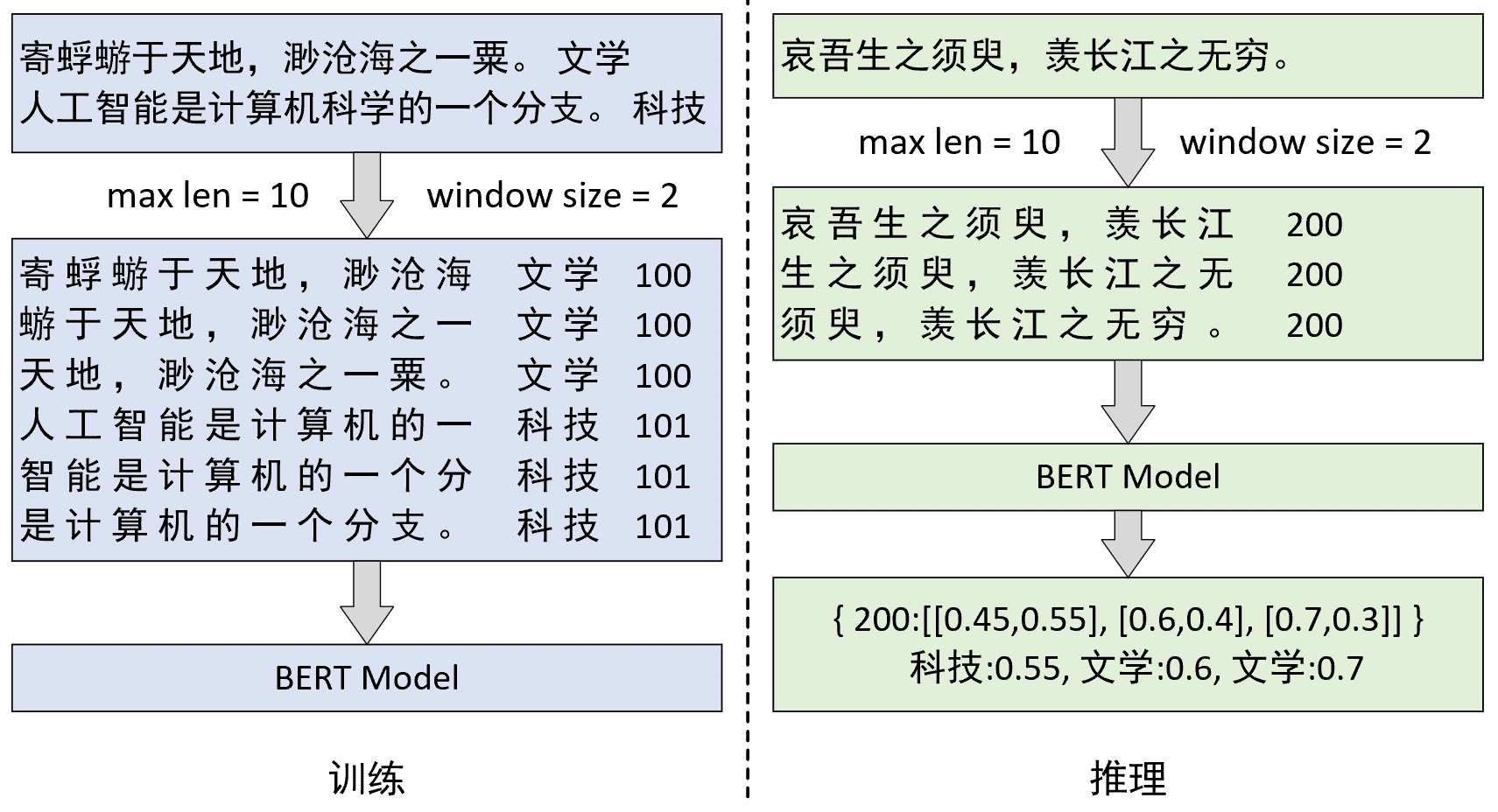
如图8-9所示便是整体的处理流程,其中左边为训练部分,右边为推理部分。在模型训练阶段时,需要先将每个原始样本按照固定长度和窗口进行滑动得到相应的子样本。例如图8-9左边的原始样本“寄蜉蝣于天地,渺沧海之一粟”就重构成了3个子样本,并且标签也同原始样本。同时,为了区分不同原始样本之间的子样本,在构造子样本时还分别加上了原始样本对应的ID。最后,将所有原始样本构造得到的子样本作为训练集来训练模型即可。
在推理阶段,对于每个原始样本来说同样要先按照训练集构造时的方式进行处理。在得到多个子样本后再分别将其进行分类并根据样本ID将同一个ID对应的所有分类结果放到一起,最后取概率最大的标签作为原始样本的预测结果即可。例如图8-9右边,“哀吾生之须臾,羡长江之无穷”这个原始样本就重构得到了3个子样本,其经过BERT分类模型后3个子样本分别被分进了“科技、文学、文学”这3个类别,最后可直接选择概率值最大的标签(文学:0.7)作为原始样本的预测值。
当然,除此之外还以将每个子样本对应的前K个概率值最大的预测结果都输出,然后再以集成模型的思想选择最终原始样本的预测结果。例如某个原始样本经过滑动窗口处理后得到5个子样本,对于每个子样本都输出前K个概率值最大的预测结果;然后可以再通过以投票的方式来决定原始样本的预测类别。
如下所示便是一段简单的滑动窗口处理示例代码可供大家参考:
 1 import numpy as np
 2 np.random.seed(2021)
 3 def data_process(samples, labels, window_size, max_len):
 4     data,uid = [],100
 5     for sample, label in zip(samples, labels):
 6         if len(sample) <= max_len:
 7             data.append([uid, sample, label])
 8             continue
 9         s_idx, e_idx = 0, max_len
10         while True:
11             s = sample[s_idx:e_idx]
12             data.append([uid, s, label])
13             if e_idx >= len(sample):
14                 break
15             s_idx += window_size
16             e_idx += window_size
17         uid += 1
18     return data
19
20 if __name__ == '__main__':
21     samples = np.random.randint(0, 100, [5, 20])
22     labels = [0, 0, 2, 1, 3]
23     print(samples)
24     data = data_process(samples, labels,window_size=6,max_len=10)
25     print(data)
在没有使用滑动窗口处理前,此时samples的输出结果如下所示:
1 [[85 57  0 94 86 44 62 91 29 21 93 24 12 70 70 33  7  1 97 26]
2  [66 48 99 63 49 16 50 54 52 93  5 49 38 14 71 85 70 41 21 25]
3  [10 36 19 57 82 90 15 40 76 53 11 19 33 78 17 89 50  7 27 63]
4  [51  9 25 71 84 27 75 27 19 31 50 89 27 18 53 32 20 95 87  3]
5  [97 20 18 70 38 90 53 62 93 26 47 91 60  7 93 33 89 37 95 48]]
在经过data_process()函数预处理之后则会变成:
1 [[100, array([85, 57,  0, 94, 86, 44, 62, 91, 29, 21]), 0],
2  [100, array([62, 91, 29, 21, 93, 24, 12, 70, 70, 33]), 0],
3  [100, array([12, 70, 70, 33,  7,  1, 97, 26]), 0],
4  [101, array([66, 48, 99, 63, 49, 16, 50, 54, 52, 93]), 0],
5  [101, array([50, 54, 52, 93,  5, 49, 38, 14, 71, 85]), 0],
6  [101, array([38, 14, 71, 85, 70, 41, 21, 25]), 0],
7  [102, array([10, 36, 19, 57, 82, 90, 15, 40, 76, 53]), 2],
8  [102, array([15, 40, 76, 53, 11, 19, 33, 78, 17, 89]), 2], ...]
到此,对于BERT中文本过长时的两种处理方法就介绍完毕了。在下一节内容中,将会详细介绍如何在PyTorch中来使用Tensorboard这一利器,以便后续更加方便的观察BERT的训练过程。